Blog

Applying a Novel Calculus Operator to Robust AI

By Amir Shachar
Lead Fraud Research Data Scientist, NICE Actimize

Here we present a new and simple operator in basic Calculus. It renders prominent deep learning frameworks and various AI applications more numerically robust. It is further advantageous in continuous domains, where it classifies trends accurately regardless of functions’ differentiability or continuity.

I used to teach my Advanced Calculus students that a function’s momentary trend is inferred from its gradient sign. Years later, in their fraud detection AI research, my employees encounter this notion often. Upon analyzing custom loss functions numerically, we treat momentary trends concisely and efficiently:

Derivative Sign

Applications

The instantaneous trend of change, embodied by the derivative sign, has been increasingly used in AI applications. Those range from optimization to computer vision and neural networks. Let’s mention some prominent examples. The “Fast Gradient Sign” method ([10], [14]) leverages the sign of the loss function’s gradient for adversarial examples generation. Further, optimization techniques that leverage the trend of change for robust and rapid convergence such as Rprop are recommended for some scenarios of deep learning ([3], [6]), and active learning ([4], [15], [26]). Prominent meta-learning frameworks such as [2], [42] leverage the gradient sign to tackle the exploding gradient problem. Memory efficient algorithms such as Quantized Stochastic Gradient Descent ([1]) and Quantized Neural Networks ([12]), quantize the gradient (where calculating its sign is a special case), and TernGrad ([39]) uses the gradient sign directly for more efficient gradient propagation. Other applications, either to explicit numeric analysis or to theorem proving, include Statistical ML ([21], [28], [32]), Neural Networks ([5], [8], [19], [20], [22], [25], [24], [29], [40]), Reinforcement Learning ([13], [16], [34]), Explainable AI ([9]), and Computer Vision ([4], [7], [11], [17], [18], [23], [27], [30], [33], [35], [41]). You’ll find a more comprehensive survey here. On top of numerical applications, the derivative sign (or that of higher-order derivatives) is traditionally applied to monotony classification tasks in continuous domains.


Points for Improvement

Numerical Robustness

Upon implementing algorithms similar to the above, consider the case where we approximate the derivative sign numerically with the difference quotient:
$$sgn\left[\frac{dL}{d\theta}\left(\theta\right)\right]\approx sgn\left[\frac{L\left(\theta+h\right)-L\left(\theta-h\right)}{2h}\right]$$This is useful for debugging your gradient computations, or in case your custom loss function, tailored by domain considerations, isn’t differentiable. The numerical issue with the gradient sign is embodied in the redundant division by a small number. It doesn’t affect the final result, the numerator, $sgn\left[L\left(\theta+h\right)-L\left(\theta-h\right)\right]$. However, it amounts to a logarithmic or linearithmic computation time in the number of digits and occasionally results in an overflow. We’d better avoid it altogether.

Analytical Robustness

Further, let’s talk about the derivative sign’s analytical application in monotony classification. We know that it often doesn’t define trend at critical points, where the derivative is zeroed or non-existent, though the function may be trending. As a simple example, consider the family of functions $f\left(x ; k\right)=\begin{cases} x^{k}, & x\neq0\\ 0, & x=0 \end{cases}$, for $k\in \mathbb{R}\backslash\left\{ 0\right\}$, and $f\left(x;k=0\right)=x^{0}\equiv1$. We illustrate some such right-derivatives at $x=0$, for different assignments of $k,$ in the following diagram. Clearly, the right-derivatives are either zeroed or equal $\infty$, for almost any selection of $k$ (except $k=1$, where the tangent coalesces with the function’s graph). However, for all $k\neq 0$, those functions increase from right throughout their definition domain, including at $x=0$. Put simply: the notion of the function’s instantaneous rate of change often doesn’t capture the instantaneous trend at critical points. Engineers work around this by calculating higher order derivatives or evaluating the function or its derivatives near the critical point. Advanced mathematical workarounds include more involved differentiation methods.

In the above example, if the derivative exists in the extended sense, then $sgn\left(\pm \infty\right) = \pm 1$ represents the function’s trend altogether. However, infinite derivatives are often considered undefined, and we should pay attention to that convention. Moreover, there are cases where the derivative doesn’t exist in the extended sense, yet the function’s trend is clear. For example, $f\left(x\right)=\begin{cases}
x+x\left|\sin\left(\frac{1}{x}\right)\right|, & x\neq0\\
0, & 0
\end{cases}$ at $x=0$. There further exist examples of various discontinuities types where the trend is clear (see below). To define the instantaneous trend of such functions we could use the sign of their (different) Dini derivatives, if we’re keen to evaluate partial limits. Otherwise, we’d like to introduce a more concise way to define trends.

Given this analysis, we’d find it convenient to have a simple operator that’s more numerically stable than the derivative sign. One that defines trends concisely and coherently whenever they’re clear, including at critical points such as discontinuities, cusps, extrema, and inflections.

The Idea

Whenever you scrutinize your car’s dashboard, you notice Calculus. The mileage is equivalent to the definite integral of the way you did so far, and the speedometer reflects the derivative of your way with respect to time. Clearly, both physical instruments merely approximate abstract notions.

Your travel direction is evidenced by the gear stick. Often, its matching mathematical concept is the derivative sign. If the car moves forward, in reverse, or freezes, then the derivative is positive, negative or zero respectively. However, calculating the derivative to evaluate its sign is occasionally superfluous. As Aristotle and Newton famously argued, nature does nothing in vain. Following their approach, to define the instantaneous trend of change, we probably needn’t go through rates calculation. Put simply: If the trend of change is a basic term in processes analysis, then perhaps we ought to reflect it concisely rather than as a by-product of the derivative?

This occasional superfluousness of the derivative causes the aforementioned issues in numeric and analytic trend classification tasks. To tackle them, we’ll attempt to simplify the derivative sign as follows:$$ \require{color}\begin{align*}
sgn\left[f_{\pm}’\left(x\right)\right] & =sgn\underset{ {\scriptscriptstyle h\rightarrow0^{\pm}}}{\lim}\left[\frac{f\left(x+h\right)-f\left(x\right)}{h}\right]\\
& \colorbox{yellow}{$\texttip{\neq}{Apply suspension of disbelief: this deliberate illegal transition contributes to the below discussion }$}\underset{ {\scriptscriptstyle h\rightarrow0^{\pm}}}{\lim}sgn\left[\frac{f\left(x+h\right)-f\left(x\right)}{h}\right]\\
& =\pm\underset{ {\scriptscriptstyle h\rightarrow0^{\pm}}}{\lim}sgn\left[f\left(x+h\right)-f\left(x\right)\right]
\end{align*}$$Note the deliberate erroneous transition in the second line. Switching the limit and the sign operators is wrong because the sign function is discontinuous at zero. Therefore the resulting operator, the limit of the sign of $\Delta y$, doesn’t always agree with the derivative sign. Further, the multiplicative nature of the sign function allows us to cancel out the division operation. Those facts may turn out in our favor, because of the issues we saw earlier with the derivative sign. Perhaps it’s worth scrutinizing the limit of the change’s sign in trend classification tasks?

This novel trend definition methodology is similar to that of the derivative. In the latter, the slope of a secant turns into a tangent as the points approach each other. In contrast, the former calculates the trend of change in an interval surrounding the point at stake, and from it deduce, by applying the limit process, the momentary trend of change. Feel free to gain intuition by hovering over the following diagram:

$\Delta y=f\left(x+\Delta x\right)-f\left(x\right)$
${\frac{\Delta y}{\Delta x}}$
$sgn\left(\Delta y\right)$

Numerical Stability

Clearly, the numerical approximations of both the (right-) derivative sign and that of $\underset{ {\scriptscriptstyle h\rightarrow0^{+}}}{\lim}sgn\left[f\left(x+h\right)-f\left(x\right)\right]$ equal the sign of the finite difference operator, $sgn\left[f\left(x+h\right)-f\left(x\right)\right]$, for some small value of $h$. However, the sign of the difference quotient goes through a redundant division by $h$. This amounts to an extra logarithmic- or linearithmic-time division computation (depending on the precision), and might result in an overflow, since $h$ is small. In that sense, we find it lucrative to think of trends approximations as $\underset{ {\scriptscriptstyle h\rightarrow0^{\pm}}}{\lim}sgn\left[f\left(x+h\right)-f\left(x\right)\right]$, rather than the derivative sign. Similar considerations lead us to apply the quantization directly to $\Delta y$ when we’re after a generic derivative quantization rather than its sign. That is, instead of quantizing the derivative, we calculate $Q\left[f\left(x+h\right)-f\left(x\right)\right]$ where $Q$ is a custom quantization function. In contrast with the trend operator, this quantization doesn’t preserve the derivative value upon skipping the division operation. However, this technique is good enough in algorithms such as gradient descent. Where the algorithmic framework entails multiplying the gradient by a constant (e.g., the learning rate), we may spare the division by $h$ in each iteration, and embody it in the pre-calculated constant itself.

A coarse estimation of the percentage of computational time spared can be achieved by considering the computations other than the trend analysis operator itself. For example, say we are able to spare a single division operation in each iteration of gradient descent. If the loss function is simple, say whose calculation is equivalent to two division operations, then we were able to spare a third of the required calculations in the process. If however the loss function is more computationally involved, for example one that includes logical operators, then the merit of sparing a division operator would be humbler.

Given this operator’s practical merit in discrete domains, let’s proceed with theoretical aspects in continuous ones.

How Does it Work

Let’s check how coherently does this operator define a local trend relative to the derivative. Recall the family of monomials from the introductory section, where we tried to define the local trend concisely by the sign of the derivative. We add another degree of freedom and allow $f\left(x ; a,k \right)=a x^k$. To gain intuition, let’s scrutinize the one-sided limit $\underset{\Delta x\rightarrow0^{+}}{\lim}sgn\left(\Delta y\right)$ and compare it to the right-derivative for cherry-picked cases. Let $k \in \left\{-1, 0, 0.5, 1, 2, 3 \right\}$, capturing discontinuity, constancy, cusp, linearity, extremum, and inflection respectively. We allow opposite values of $a$ to cover all types of trends. Feel free to tweak the following radio buttons and observe the limit process in action for both operators:
Select Metric


Select $a$


Select $k$

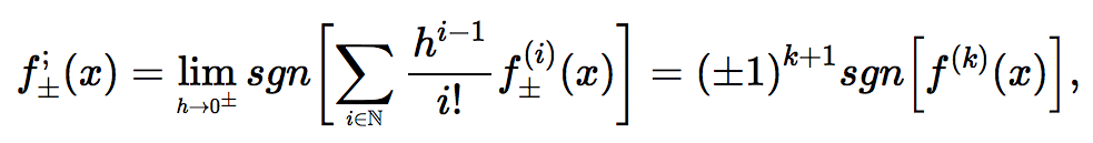
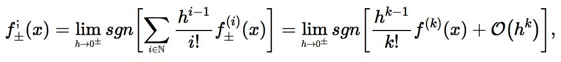
As we’ve seen, in all those cases, $\underset{\Delta x\rightarrow0^{+}}{\lim}sgn\left(\Delta y\right)$ reflects the way we think about the trend: it always equals $a$ except for the constancy case, where it’s zeroed, as expected. It’s possible to show it directly with limit Calculus, see some examples below. We also concluded in the introductory section that the derivative sign doesn’t capture momentary trends except for $k\in \left\{0,1\right\}$. We gather that this operator does better in capturing trends at critical points.

Why Does it Work

We can establish a more rigorous justification by noticing how the definition of local extrema points coalesces with that of the operator at stake. In contrast with its basic Calculus analog, the following claim provides both a sufficient and necessary condition for stationary points:

Theorem 1. Analog to Fermat’s Stationary Point Theorem. Let $f:\left(a,b\right)\rightarrow\mathbb{R}$ be a function and let $x\in \left(a,b\right).$ The following condition is necessary and sufficient for $x$ to be a strict local extremum of $f$:

$$\exists \underset{h\rightarrow0}{\lim}sgn\left[f\left(x+h\right)-f\left(x\right)\right]\neq0.$$

The avid Calculus reader will notice that this theorem immediately follows from the Cauchy limit definition.

Without loss of generality, we will prove the theorem for maxima points. We show that the following definitions of local extrema are equivalent: $$\begin{array}{ccc} & \exists\delta>0:\left|x-\bar{x}\right|<\delta\Longrightarrow f\left(x\right)>f\left(\bar{x}\right)\\ & \Updownarrow\\ & \underset{ {\scriptscriptstyle h\rightarrow0^{\pm}}}{\lim}sgn\left[f\left(x+h\right)-f\left(x\right)\right]=-1 \end{array}$$ First direction. Assume $$\underset{ {\scriptscriptstyle h\rightarrow0^{\pm}}}{\lim}sgn\left[f \left(x+h\right)-f\left(x\right)\right]=-1.$$ Then according to Cauchy limit definition, $$\forall\epsilon,\exists\delta:\left|x-\bar{x}\right| < \delta\Longrightarrow\left|sgn\left[f\left(\bar{x}\right)-f\left(x\right)\right]-\left(-1\right)\right| < \epsilon.$$ In particular, for $\epsilon_{0}=\frac{1}{2}$, $$\exists\delta:\left|x-\bar{x}\right|<\delta\Longrightarrow\left|sgn\left[f\left(\bar{x}\right)-f\left(x\right)\right]+1\right|<\frac{1}{2}.$$ The only value in the sign function’s image, $\left\{ 0,\pm1\right\}$, that satisfies the above inequality, is $-1$. Therefore: $$\exists\delta:\left|x-\bar{x}\right|<\delta\Longrightarrow sgn\left[f\left(\bar{x}\right)-f\left(x\right)\right]=-1,$$ which can be written as: $$\exists\delta:\left|x-\bar{x}\right|<\delta\Longrightarrow f\left(x\right)>f\left(\bar{x}\right).$$ Second direction. Let $\epsilon>0$. We know that there exists $\delta$ such that $\left|x-\bar{x}\right| < \delta$ implies that $f\left(x\right)>f\left(\bar{x}\right)$, which can be rewritten as $$sgn\left[f\left(\bar{x}\right)-f\left(x\right)\right]=-1.$$ Thus $sgn\left[f\left(\bar{x}\right)-f\left(x\right)\right]-\left(-1\right)=0$, and in particular $$\left|sgn\left[f\left(\bar{x}\right)-f\left(x\right)\right]-\left(-1\right)\right|<\epsilon,$$ and the limit definition holds. $\blacksquare$

Feel free to scrutinize the relation between the Semi-discrete and the continuous versions of Fermat’s theorem in the following animation:

Where Does it Work

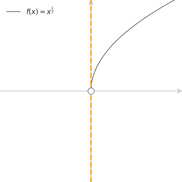
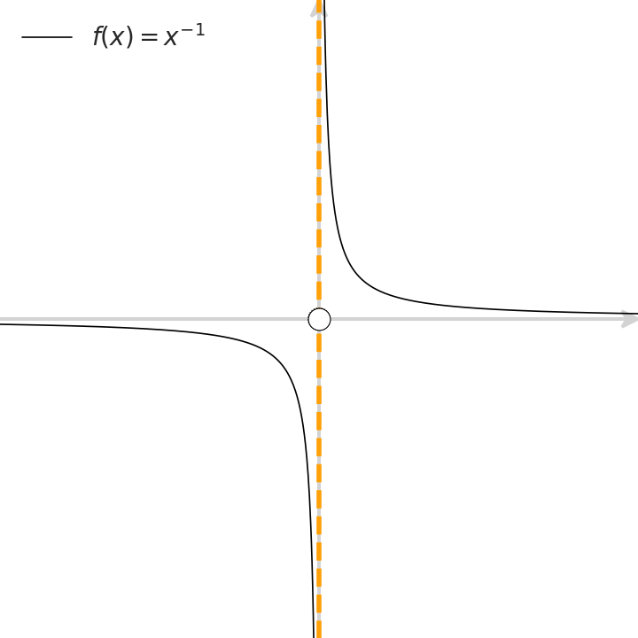
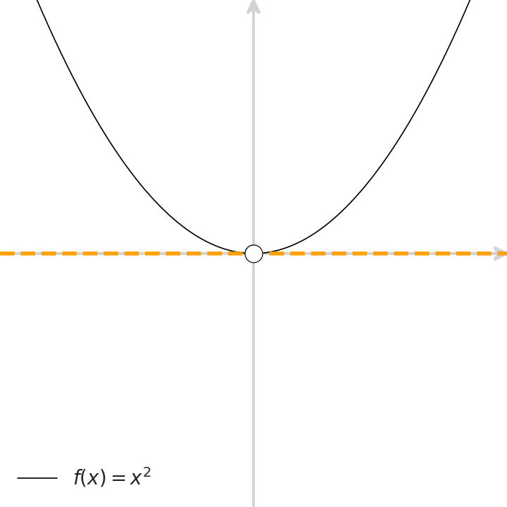
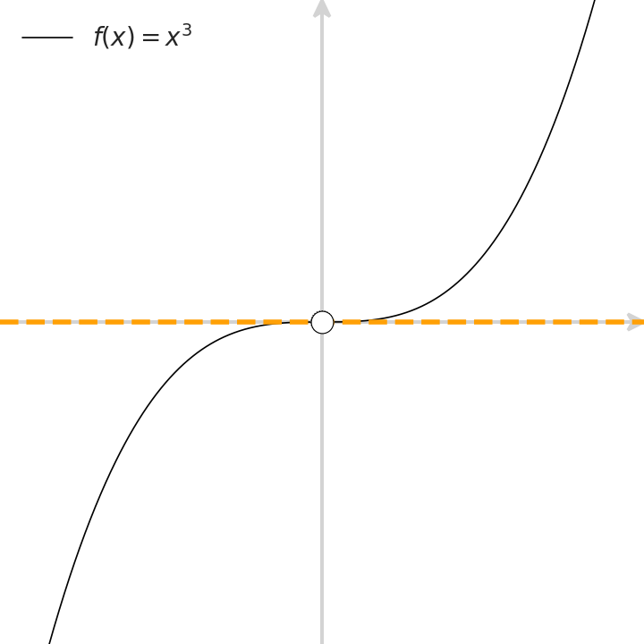
Next, let’s check in which scenarios is this operator well defined. We’ll cherry-pick functions with different characteristics around $x=0$. For each such function, we ask which of the properties (continuity, differentiability, and the existence of the operator at stake, that is, the existence of a local trend from both sides), take place at $x=0$. Scrutinize the following animation to gain intuition with some basic examples:

We would also like to find out which of those properties hold across an entire interval (for example, $[-1,1]$). To that end, we add two interval-related properties: Lebesgue and Riemann integrability. Feel free to explore those properties in the following widget, where we introduce slightly more involved examples than in the above animation. Switch between the granularity levels, and hover over the sections or click on the functions in the table, to confirm which conditions hold at each case:

Select Granularity
Function
$f_1\left(x\right)=x^2$
$f_2\left(x\right)=\left(\frac{1}{2}-\boldsymbol{1}_{\mathbb{Q}}\right)x^{2}$
$f_3\left(x\right)=x^{\frac{1}{3}}$
$f_4\left(x\right)=t\left(x-\sqrt{2}\right),$
where $t$ is Thomae's function
$f_5\left(x\right)=sgn\left(x\right)$
$f_6\left(x\right)=\begin{cases} \sin\left(\frac{1}{x}\right), & x\neq0\\ 0, & x=0 \end{cases}$
$f_7\left(x\right)= x^{1+2\cdot\boldsymbol{1}_{\mathbb{Q}}}$
$f_8\left(x\right)=R\left(x\right),$
where $R$ is Riemann function ([43])
$f_{9}\left(x\right)=\begin{cases} \sin\left(\frac{1}{x}\right), & x\neq0\\ 2, & x=0 \end{cases}$


Function
$f_1\left(x\right)=\boldsymbol{1}_{\mathbb{Q}}$ (Dirichlet)
$f_2\left(x\right)=\begin{cases} \sin\left(\frac{1}{x}\right), & x\neq0\\ 0.5, & x=0 \end{cases}$
$f_3\left(x\right)=\begin{cases} \sin\left(\frac{1}{x}\right), & x\neq0\\ 0, & x=0 \end{cases}$
$f_4\left(x\right)=\begin{cases} x^2\sin\left(\frac{1}{x}\right), & x\neq0\\ 0, & x=0 \end{cases}$
$f_5\left(x\right)=x$
$f_6\left(x\right)=\sqrt{\left|x\right|}$
$f_{7}\left(x\right)=sgn\left(x\right)$
$f_{8}\left(x\right)=\begin{cases} \frac{1}{\sqrt{\left|x\right|}}, & x\neq0\\ 0, & x=0 \end{cases}$
$f_{9}\left(x\right)=\begin{cases} \frac{1}{x}, & x\neq0\\ 0, & x=0 \end{cases}$


We may extend the discussion to properties that hold in intervals almost everywhere, rather than throughout the interval. This is out of this article’s scope, but as a taste we’ll mention the function $f(x)=\sum\limits_{n=1}^{\infty}f_n(x)$, where $f_n(x)=2^{-n}\phi\left(\frac{x-a_n}{b_n-a_n}\right), \phi$ is the Cantor-Vitali function and $\{(a_n,b_n):n\in\mathbb{N}\}$ is the set of all intervals in $\left[0,1\right]$ with rational endpoints. It’s possible to show that this function has trend everywhere, it’s strictly monotonic, but its derivative is zeroed almost everywhere. In this example, the notion of instantaneous trend is coherent with the function’s monotonic behavior in the interval, in contrast with the vanishing derivative. Further, according to Baire categorization theorem, almost all the continuous functions are nowhere differentiable. Therefore, we could use an extension to the set of functions whose monotony can be analyzed concisely. Finally, we mention the function $g\left(x\right)=x^{1+\boldsymbol{1}_{\mathbb{Q}}}$ defined over $\left(0,1\right)$. In its definition domain, $g$ is discontinuous everywhere, but detachable from left almost everywhere.

Defining the Instantaneous Trend of Change

Let’s summarize our discussion thus far. The momentary trend, a basic analytical concept, has been embodied by the derivative sign for engineering purposes. It’s applied to constitutive numeric algorithms across AI, optimization and other computerized applications. More often than not, it doesn’t capture the momentary trend of change at critical points. In contrast, $\underset{\Delta x\rightarrow0^{\pm}}{\lim}sgn\left(\Delta y\right)$ is more numerically robust, in terms of finite differences. It defines trends coherently wherever they exist, including at critical points. Given those merits, why don’t we dedicate a definition to this operator? As it “detaches” functions, turning them into step functions with discontinuities at extrema points, let’s define the one-sided detachments of a function $f$ as follows:

We say that a function is detachable if both those one-sided limits exist. We add the $\pm$ coefficient for consistency with the derivative sign. For convenience and brevity, from now on we denote by $f^;$ either one of the one-sided detachments separately ($f^;_+$ or $f^;_-$), while not assuming that they necessarily agree.

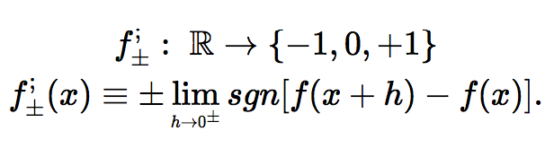
Geometrically speaking, for a function’s (right-) detachment to equal $+1$ for example, its value at the point needs to strictly bound the function’s values in a right-neighborhood of $x$ from below. This is in contrast with the derivative’s sign, where the assumption on the existence of an ascending tangent is made.

Feel free to scrutinize the logical steps that led to the definition of the detachment from the derivative sign in the following animation (created with Manim):

Single Variable Semi-discrete Calculus

Equipped with a concise definition of the instantaneous trend of change, we may formulate analogs to Calculus theorems with the following trade-off. Those simple corollaries inform us of the function’s trend rather than its rate. In return, they hold for a broad set of detachable and non-differentiable functions. They are also outlined in [31].

Simple Algebraic Properties

Claim 2. Constant Multiple Rule. If $f$ is detachable at $x$, and $c\in \mathbb{R}$ is a constant, then $cf$ is also detachable and the following holds there: $$\left(cf\right)^{;}=sgn\left(cf^{;}\right).$$

$$\left(cf\right)_{\pm}^{;} = \pm \underset{t\rightarrow x^{\pm}}{\lim}sgn\left[\left(cf\right)\left(x+h\right)-\left(cf\right)\left(x\right)\right] = \pm \underset{t\rightarrow x^{\pm}}{\lim}sgn\left(c\right)sgn\left[f\left(x+h\right)-f\left(x\right)\right]=sgn\left(c\right)f_{\pm}^{;}=sgn\left[cf_{\pm}^{;}\right].\,\,\,\,\blacksquare$$

Claim 3. Sum and Difference Rules. If $f$ and $g$ are detachable at $x$ and $\left(f^{;} g^{;} \right) \left(x\right) \in \left\{0, \pm 1 \right \}$ (the plus or minus signs are for the sum and difference rules, respectively), then the following holds at $x$:

$$\left(f \pm g\right)^{;}=sgn\left( f^{;} \pm g^{;} \right).$$

Without loss of generality, let’s focus on right-detachments. We’ll show that if $f^{;}_{+}\left(x\right)=g^{;}_{+}\left(x\right)$ then $\left(f+g\right)^{;}_{+}\left(x\right)=+1$, and the rest of the cases are proved similarly. There exists a right-neighborhood bounded by $\delta_{f}$ where: $$0<\bar{x}-x<\delta_{f}\Longrightarrow sgn\left[f\left(\bar{x}\right)-f\left(x\right)\right]=+1\Longrightarrow f\left(\bar{x}\right) > f\left(x\right).$$ Similarly there exists a right-neighborhood bounded by $\delta_{g}$ where: $$0<\bar{x}-x<\delta_{g}\Longrightarrow g\left(\bar{x}\right) > g\left(x\right).$$ Therefore there exists a right-neighborhood bounded by $\delta_{f+g}\equiv\min\left\{ \delta_{f},\delta_{g}\right\}$ where: $$0<\bar{x}-x<\delta_{f+g}:\,\, sgn\left[\left(f+g\right)\left(\bar{x}\right)-\left(f+g\right)\left(x\right)\right]=+1,$$ hence $$\underset{\bar{x}\rightarrow x^{+}}{\lim}sgn\left[\left(f+g\right)\left(\bar{x}\right)-\left(f+g\right)\left(x\right)\right]=+1. \,\,\,\,\blacksquare$$

Claim 4. If $f$, $g$ and $f+g$ are detachable at $x$, and the one-sided detachments of $f$ and $g$ aren’t both zeroed there, then the following holds at $x$:

$$f^{;}g^{;}=\left(f+g\right)^{;}\left(f^{;}+g^{;}\right)-1.$$

It is possible to show by separating to cases that for $A,B$ not both zero:$$sgn\left(A\right)sgn\left(B\right)=sgn\left(A+B\right)\left[sgn\left(A\right)+sgn\left(B\right)\right]-1.$$The result is obtained by taking $A=f\left(x+h\right)-f\left(x\right)$ and $B=g\left(x+h\right)-g\left(x\right)$, followed by applying the one-sided limit process to both sides.$\,\,\,\,\blacksquare$

Don’t worry about the sum rule holding only for functions whose detachments aren’t additive inverses. We will handle those cases, assuming differentiability, later on with Taylor series.

Product and Quotient Rules

Let’s begin this discussion with a simple example. If $f^{;}=g^{;}=+1$, and $f=g=0$ at a point $x$, then the detachment of the product is $\left(fg\right)^{;}=+1$ as well. Following this simple scenario, one might be tempted to think that the product rule for the detachment is simply $\left(fg\right)^{;}=f^{;}g^{;}$. However, upon shifting $g$ vertically downwards, that is, requiring that $g(x)<0$, we obtain a setting where $\left(fg\right)^{;}=-1$, and that’s although the detachments of $f,g$ remained as before. It means that the detachment of the product $\left(fg\right)^{;}$ necessarily depends also on the sign of $f,g$ at the point of interest. Indeed, assuming $g$ is continuous we have that the product’s detachment is $-1$ in this new setting.

However, let us recall that in Semi-discrete Calculus we aren’t restricted to differentiable or even continuous functions. What if $g$ is discontinuous? As long as $g$ maintains its sign in the neighborhood of the point, it’s possible to show that the detachment of the product remains $-1$. But if $g$ changes its sign, meaning there exists a neighborhood of $x$ where $g$ is zeroed or one where $g$ is positive, then $\left(fg\right)^{;}$ can be either $0$ or $+1$ respectively. This implies that we should somehow bound the functions’ signs. I suggest to pay attention to an intuitive trait of the functions $f,g$: sign-continuity.

Given a function $f$, we will say that it is sign-continuous (s.c.) at a point $x$ if $sgn\left(f\right)$ is continuous there. If all the partial limits of $sgn\left(f\right)$ are different than its sign at $x$, then we will say that $f$ is sign-discontinuous (s.d.) there. Observe that the function’s sign-continuity at a point may be determined given its sign and detachment there. That is, if $f^{;}=0$ or $ff^{;}>0$, then $f$ is sign-continuous. We will say that $f$ is inherently sign-continuous (i.s.c.) in such cases. In contrast, if $f^{;}\neq0$ and $f=0$, or $ff^{;}<0$, then $f$ is inherently sign-discontinuous (i.s.d).

A function that is either sign-continuous or sign-discontinuous will be called sign-consistent. We restrict ourselves in the following discussion to sign-consistent functions.

In the process of formulating the product rule, we repeatedly conduct analyses similar to the above, with different combinations of $f^{;},g^{;}$, their signs, and assumptions on their sign-continuity or lack thereof.

You’ll find here a simulation code for the creation of the data required to extract those rules. The final results obtained from the simulation are also available, in two separate Google sheets, here.

In each of those many cases, we conduct an $\epsilon-\delta$ analysis and prove that the product’s detachment equals a value, in case it’s indeed determined.

Recall that the product rule for derivatives dictates the following combination of the original functions’ derivatives: $\left(fg\right)’=f’g+fg’$. Evidently, the results we gather regarding the detachments product follow a similar rule in part of the cases and another intuitive formula in others. Recall that the following product and quotient rules hold for detachable, not necessarily continuous functions.

Claim 5. Product Rule. Let $f$ and $g$ be detachable and sign-consistent at $x$. If one of the following holds there:

    1. $ff^{;}gg^{;}\geq0$, where $f$ or $g$ is s.c. or $f=g=0$
    2. $ff^{;}gg^{;}<0$, where $f$ or $g$ is s.d.

Then $fg$ is detachable there, and: $$\left(fg\right)^{;}=\begin{cases}
sgn\left[f^{;}sgn\left(g\right)+g^{;}sgn\left(f\right)\right], & ff^{;}gg^{;}\geq0\text{, and }f\text{ or }g\text{ is s.c.}\\
f^{;}g^{;}, & \text{else}\text{.}
\end{cases}$$

For brevity, we will refer to the terms $sgn\left[f^{;}sgn\left(g\right)+g^{;}sgn\left(f\right)\right]$ and $f^{;}g^{;}$ from the theorem statement as the first and second formulas, respectively. Let us distinguish between the following cases, according to the pointwise signs of $f,g$ and their detachments there (the vector $\left(f^{;},sgn\left(f\right),g^{;},sgn\left(g\right)\right)\in\left\{ \pm1,0\right\} ^{4}$), and their inherent sign-continuity or lack thereof.
    1. Assume $ff^{;}gg^{;}>0$. There are 8 such combinations of $\left(f^{;},sgn\left(f\right),g^{;},sgn\left(g\right)\right)$:
      • Assume that either $f$ or $g$ is inherently sign-continuous. There are 4 such cases, in which both $f,g$ adhere to the inherent sign-continuity property. Without loss of generality assume that $f^{;}=g^{;}=sgn\left(f\right)=sgn\left(g\right)=+1$. Then: $$\begin{cases} \exists\delta_{f}: & \forall\bar{x}\in B_{\delta_{f}}\left(x\right):f\left(\bar{x}\right)>f\left(x\right)>0\\ \exists\delta_{g}: & \forall\bar{x}\in B_{\delta_{g}}\left(x\right):g\left(\bar{x}\right)>g\left(x\right)>0 \end{cases}$$ hence for $\delta_{fg}\equiv\min\left\{ \delta_{f},\delta_{g}\right\}$ it holds that: $$\forall\bar{x}\in B_{\delta_{fg}}\left(x\right):\left(fg\right)\left(\bar{x}\right)=f\left(\bar{x}\right)g\left(\bar{x}\right)>f\left(x\right)g\left(x\right)=\left(fg\right)\left(x\right),$$ and $\left(fg\right)^{;}\left(x\right)=+1=sgn\left[\left(+1\right)\cdot\left(+1\right)+\left(+1\right)\cdot\left(+1\right)\right]$, in accordance with the second formula.
      • Assume that neither $f$ nor $g$ is inherently sign-continuous. There are 4 such cases. Without loss of generality assume that $f^{;}=g^{;}=+1$ and $f,g<0$. Then: $$\begin{cases} \exists\delta_{f}^{\left(1\right)}: & \forall\bar{x}\in B_{\delta_{f}^{\left(1\right)}}\left(x\right):f\left(\bar{x}\right)>f\left(x\right)\\ \exists\delta_{g}: & \forall\bar{x}\in B_{\delta_{g}}\left(x\right):g\left(\bar{x}\right)>g\left(x\right)\\ & f\left(x\right)<0\\ & g\left(x\right)<0 \end{cases}$$ The continuity of $sgn\left(f\right)$ cannot be inferred directly from the definition of the detachment and its value’s sign there. Therefore, we will assume that $f$ is sign-continuous explicitly: $$\exists\delta_{f}^{\left(2\right)}:\forall\bar{x}\in B_{\delta_{f}^{\left(2\right)}}\left(x\right):f\left(\bar{x}\right)<0,$$ hence for $\delta_{fg}\equiv\min\left\{ \delta_{f^{\left(1\right)}},\delta_{f^{\left(2\right)}},\delta_{g}\right\}$ it holds that: $$\forall\bar{x}\in B_{\delta_{fg}}\left(x\right): \left(fg\right)\left(\bar{x}\right)=f\left(\bar{x}\right)g\left(\bar{x}\right) < f\left(\bar{x}\right)g\left(x\right) < f\left(x\right)g\left(x\right)=\left(fg\right)\left(x\right),$$ and $\left(fg\right)^{;}\left(x\right)=-1=sgn\left[\left(+1\right)\cdot\left(-1\right)+\left(+1\right)\cdot\left(-1\right)\right]$, in accordance with the second formula.
    2. Assume $ff^{;}gg^{;}=0$. There are 65 such combinations of $\left(f^{;},sgn\left(f\right),g^{;},sgn\left(g\right)\right)$:
      • Assume that $f$ or $g$ is sign-continuous. There are 61 such combinations:
        • Assume that one of $f,g$ is inherently sign-continuous and the other is inherently sign-discontinuous. There are 20 such combinations of $\left(f^{;},sgn\left(f\right),g^{;},sgn\left(g\right)\right)$. Without loss of generality, assume that $f^{;}=g^{;}=-1,f<0$ and $g=0$, where $f$ is inherently sign-continuous and $g$ is inherently sign-discontinuous. Then: $$\begin{cases} \exists\delta_{f}: & \forall\bar{x}\in B_{\delta_{f}}\left(x\right):f\left(\bar{x}\right) < f\left(x\right) < 0\\ \exists\delta_{g}: & \forall\bar{x}\in B_{\delta_{g}}\left(x\right):g\left(\bar{x}\right) < g\left(x\right)=0 \end{cases}$$ hence for $\delta_{fg}\equiv\min\left\{ \delta_{f},\delta_{g}\right\}$ it holds that: $$\forall\bar{x}\in B_{\delta_{fg}}\left(x\right):\left(fg\right)\left(\bar{x}\right)=f\left(\bar{x}\right)g\left(\bar{x}\right) > 0=\left(fg\right)\left(x\right),$$ and $\left(fg\right)^{;}\left(x\right)=+1=sgn\left[\left(-1\right)\cdot0+\left(-1\right)\cdot\left(-1\right)\right]$, in accordance with the second formula.
        • Assume that one of $f,g$ is inherently sign-continuous and the other is neither inherently sign-continuous nor inherently sign-discontinuous. There are 12 such combinations of $\left(f^{;},sgn\left(f\right),g^{;},sgn\left(g\right)\right)$. Without loss of generality, assume that $f^{;}=0,g^{;}=-1,f < 0$ and $g > 0$, where $f$ is inherently sign-continuous. Then: $$\begin{cases} \exists\delta_{f}: & \forall\bar{x}\in B_{\delta_{f}}\left(x\right):f\left(\bar{x}\right)=f\left(x\right) < 0\\ \exists\delta_{g}: & \forall\bar{x}\in B_{\delta_{g}}\left(x\right):g\left(\bar{x}\right)< g\left(x\right)\\ & g\left(x\right) > 0 \end{cases}$$ hence for $\delta_{fg}\equiv\min\left\{ \delta_{f},\delta_{g}\right\}$ it holds that: $$\forall\bar{x}\in B_{\delta_{fg}}\left(x\right):\left(fg\right)\left(\bar{x}\right)=f\left(\bar{x}\right)g\left(\bar{x}\right) > f\left(x\right)g\left(x\right)=\left(fg\right)\left(x\right),$$ and $\left(fg\right)^{;}\left(x\right)=+1=sgn\left[\left(0\right)\cdot\left(+1\right)+\left(-1\right)\cdot\left(-1\right)\right],$ in accordance with the second formula.
        • Assume that one of $f,g$ is inherently sign-discontinuous and the other is neither inherently sign-continuous nor inherently sign-discontinuous. There are 8 such combinations of $\left(f^{;},sgn\left(f\right),g^{;},sgn\left(g\right)\right)$. Without loss of generality, assume that $f^{;}=g^{;}=-1,f>0$ and $g=0$, where $g$ is inherently sign-discontinuous and $f$ is neither inherently sign-continuous nor sign-discontinuous. Then: $$\begin{cases} \exists\delta_{f^{\left(1\right)}}: & \forall\bar{x}\in B_{\delta_{f}^{\left(1\right)}}\left(x\right):f\left(\bar{x}\right) < f\left(x\right) < 0\\ \exists\delta_{g}: & \forall\bar{x}\in B_{\delta_{g}}\left(x\right):g\left(\bar{x}\right) < g\left(x\right)=0 \end{cases}$$ Let’s assume the continuity of $f$ at $x$ explicitly: $\exists\delta_{f^{\left(2\right)}}:\forall\bar{x}\in B_{\delta_{f}^{\left(2\right)}}\left(x\right):f\left(\bar{x}\right) < 0,$ hence for $\delta_{fg}\equiv\min\left\{ \delta_{f}^{\left(1\right)},\delta_{f}^{\left(2\right)},\delta_{g}\right\}$ it holds that: $$\forall\bar{x}\in B_{\delta_{fg}}\left(x\right):\left(fg\right)\left(\bar{x}\right)=f\left(\bar{x}\right)g\left(\bar{x}\right)< 0=\left(fg\right)\left(x\right),$$ and $\left(fg\right)^{;}\left(x\right)=-1=sgn\left[\left(-1\right)\cdot0+\left(-1\right)\cdot\left(+1\right)\right]$, in accordance with the second formula.
        • Assume that both $f,g$ are inherently sign-continuous. There are 21 such combinations of $\left(f^{;},sgn\left(f\right),g^{;},sgn\left(g\right)\right)$. Without loss of generality, assume that $f^{;}=g^{;}=0,f< 0$ and $g<0$, where $f,g$ are both inherently sign-continuous. Then: $$\begin{cases} \exists\delta_{f}: & \forall\bar{x}\in B_{\delta_{f}}\left(x\right):f\left(\bar{x}\right)=f\left(x\right)< 0\\ \exists\delta_{g}: & \forall\bar{x}\in B_{\delta_{g}}\left(x\right):g\left(\bar{x}\right)< g\left(x\right)<0 \end{cases}$$ hence for $\delta_{fg}\equiv\min\left\{ \delta_{f},\delta_{g}\right\}$ it holds that: $$\forall\bar{x}\in B_{\delta_{fg}}\left(x\right):\left(fg\right)\left(\bar{x}\right)=f\left(\bar{x}\right)g\left(\bar{x}\right) > f\left(x\right)g\left(x\right)=\left(fg\right)\left(x\right),$$ and $\left(fg\right)^{;}\left(x\right)=0=sgn\left[\left(0\right)\cdot\left(-1\right)+\left(0\right)\cdot\left(-1\right)\right]$, in accordance with the second formula.
      • Assume that $f=g=0$. There are 4 such combinations of $\left(f^{;},sgn\left(f\right),g^{;},sgn\left(g\right)\right)$. In these cases, both $f,g$ are inherently sign-discontinuous. Without loss of generality, assume that $f^{;}=g^{;}=1,f=g=0$, where $f,g$ are both inherently sign-discontinuous. Then: $$\begin{cases} \exists\delta_{f}: & \forall\bar{x}\in B_{\delta_{f}}\left(x\right):f\left(\bar{x}\right)< f\left(x\right)=0\\ \exists\delta_{g}: & \forall\bar{x}\in B_{\delta_{g}}\left(x\right):g\left(\bar{x}\right)< g\left(x\right)=0 \end{cases}$$ hence for $\delta_{fg}\equiv\min\left\{ \delta_{f},\delta_{g}\right\}$ it holds that: $$\forall\bar{x}\in B_{\delta_{fg}}\left(x\right):\left(fg\right)\left(\bar{x}\right)=f\left(\bar{x}\right)g\left(\bar{x}\right)> 0=f\left(x\right)g\left(x\right)=\left(fg\right)\left(x\right),$$ and $\left(fg\right)^{;}\left(x\right)=+1=\left(+1\right)\cdot\left(+1\right)$, in accordance with the first formula.
    3. Assume $ff^{;}gg^{;}<0$. There are 8 such combinations of $\left(f^{;},sgn\left(f\right),g^{;},sgn\left(g\right)\right)$. For each combination it holds that $ff^{;}>0$ or $gg^{;}>0$, hence either $f$ or $g$ is inherently sign-continuous. Without loss of generality assume that $f^{;}=+1,f>0,g^{;}=-1$ and $g>0$. Then: $$\begin{cases} \exists\delta_{f}: & \forall\bar{x}\in B_{\delta_{f}^{\left(1\right)}}\left(x\right):f\left(\bar{x}\right) > f\left(x\right) >0\\ \exists\delta_{g}^{\left(1\right)}: & \forall\bar{x}\in B_{\delta_{g}}\left(x\right):g\left(\bar{x}\right)< g\left(x\right)\\ & g\left(x\right)>0 \end{cases}$$ The continuity of $sgn\left(f\right)$ can be inferred directly from the definition of the detachment and its value’s sign there. However, $g$ is neither inherently sign-continuous nor inhrently sign-discontinuous. Thus we will assume that $g$ is sign-discontinuous explicitly: $$\exists\delta_{g}^{\left(2\right)}:\forall\bar{x}\in B_{\delta_{g}^{\left(2\right)}}\left(x\right):g\left(\bar{x}\right)\leq0,$$ hence for $\delta_{fg}\equiv\min\left\{ \delta_{f},\delta_{g^{\left(1\right)}},\delta_{g^{\left(2\right)}}\right\}$ it holds that: $$\forall\bar{x}\in B_{\delta_{fg}}\left(x\right):\left(fg\right)\left(\bar{x}\right)=f\left(\bar{x}\right)g\left(\bar{x}\right)\leq0 < f\left(x\right)g\left(x\right)=\left(fg\right)\left(x\right),$$ and $\left(fg\right)^{;}\left(x\right)=-1=\left(+1\right)\cdot\left(-1\right)$, in accordance with the first formula.$\,\,\,\,\blacksquare$

Claim 6. Quotient Rule. Let $f$ and $g$ be detachable and sign-consistent at $x$, where $g\neq0$ across their definition domain. Assume that $f,g$ are either s.c. or s.d. If one of the following holds there:

    1. $ff^{;}gg^{;}\leq0$, where $f$ or $g$ is s.c., or $f=0$
    2. $ff^{;}gg^{;}>0$, where only one of $f,g$ is s.c.

Then $\frac{f}{g}$ is detachable there, and: $$\left(\frac{f}{g}\right)^{;}=\begin{cases}
sgn\left[f^{;}sgn\left(g\right)-g^{;}sgn\left(f\right)\right], & g\text{ is i.s.c., or }f\text{ and }g\text{ are s.c.},\text{or }f=0\text{ and }f\text{ or }g\text{ is s.c.}\\
sgn\left[f^{;}sgn\left(g\right)+g^{;}sgn\left(f\right)\right], & \text{else if }ff^{;}gg^{;}\geq0\text{, and }f\text{ or }g\text{ is s.c.}\\
f^{;}g^{;}, & \text{else.}
\end{cases}$$

For brevity, we will refer to the terms $sgn\left[f^{;}sgn\left(g\right)-g^{;}sgn\left(f\right)\right]$, $sgn\left[f^{;}sgn\left(g\right)+g^{;}sgn\left(f\right)\right]$ and $f^{;}g^{;}$ from the theorem statement as the first, second and third formulas and conditions, respectively. We prove the claim by separating to cases. We will suggest here a slightly shorter analysis with respect to the proof of the product rule, as the ideas are similar. We will survey here a handful of representative cases. The rest of them are shown to hold analogously.
    1. Assume that $g$ is i.s.c. Without lose of generality, assume $f^{;}=g^{;}=-1,f>0$ and $g<0$. There are two cases: either $f$ is s.d., or it is s.c.
      • Assuming $f$ is s.d., then:$$\begin{cases}\exists\delta_{f}^{\left(1\right)}: & \forall\bar{x}\in B_{\delta_{f}^{\left(1\right)}}\left(x\right):f\left(\bar{x}\right)< f\left(x\right)\\\exists\delta_{f}^{\left(2\right)}: & \forall\bar{x}\in B_{\delta_{f}^{\left(2\right)}}\left(x\right):f\left(\bar{x}\right)\leq0\\\exists\delta_{g}: & \forall\bar{x}\in B_{\delta_{g}}\left(x\right):g\left(\bar{x}\right)< g\left(x\right)\\ & f\left(x\right)>0\\& g\left(x\right)<0,\end{cases}$$hence for $\delta_{f/g}\equiv\min\left\{ \delta_{f}^{\left(1\right)},\delta_{f}^{\left(2\right)},\delta_{g}\right\}$ it holds that:$$\forall\bar{x}\in B_{\delta_{f/g}}\left(x\right):\frac{f}{g}\left(\bar{x}\right)\in\left\{ 0,+1\right\},$$however $\frac{f}{g}\left(x\right)<0$, therefore $sgn\left[\frac{f}{g}\left(\bar{x}\right)-\frac{f}{g}\left(x\right)\right]=+1$ in a neighborhood of $x$. Thus $\left(\frac{f}{g}\right)^{;}\left(x\right)=+1=sgn\left[\left(-1\right)\cdot\left(-1\right)-\left(-1\right)\cdot\left(+1\right)\right]$, in accordance with the first formula.
      • Assuming $f$ is s.c. while maintaining the conditions in the previous example, we have: $$\exists\tilde{\delta}_{f}^{\left(2\right)}:\forall\bar{x}\in B_{\tilde{\delta}_{f}^{\left(2\right)}}\left(x\right):f\left(\bar{x}\right)>0,$$hence for $\tilde{\delta}{}_{f/g}\equiv\min\left\{ \delta_{f}^{\left(1\right)},\tilde{\delta}_{f}^{\left(2\right)},\delta_{g}\right\}$ it holds that:$$\forall\bar{x}\in B_{\delta_{f/g}}\left(\bar{x}\right):\left|\frac{f}{g}\left(\bar{x}\right)\right|<\left|\frac{f}{g}\left(x\right)\right|,$$ and since $\frac{f}{g}\left(\bar{x}\right),\frac{f}{g}\left(x\right)$ are both negative then $\frac{f}{g}\left(\bar{x}\right)>\frac{f}{g}\left(x\right)$ in that neighborhood of $x$, and again $\left(\frac{f}{g}\right)^{;}\left(x\right)=+1$.
    2. Assume that $f,g$ are both s.c. Without lose of generality, assume $f^{;}=g^{;}=-1,f<0$ and $g>0$. Then $f$ is i.s.c., and we will impose the assumption that $g$ is s.c. Then:$$\begin{cases}\exists\delta_{f}: & \forall\bar{x}\in B_{\delta_{f}}\left(x\right):f\left(\bar{x}\right)< f\left(x\right)\\ \exists\delta_{g}^{\left(1\right)}: & \forall\bar{x}\in B_{\delta_{g}^{\left(1\right)}}\left(x\right):g\left(\bar{x}\right)\leq g\left(x\right)\\ \exists\delta_{g}^{\left(2\right)}: & \forall\bar{x}\in B_{\delta_{g}^{\left(2\right)}}\left(x\right):g\left(\bar{x}\right)>0\\& f\left(x\right)>0\\& g\left(x\right)<0, \end{cases}$$ hence for $\delta_{f/g}\equiv\min\left\{ \delta_{f},\delta_{g}^{\left(1\right)},\delta_{g}^{\left(2\right)}\right\}$ it holds that: $$\forall\bar{x}\in B_{\delta_{f/g}}\left(x\right):\left|\frac{f}{g}\left(\bar{x}\right)\right|>\left|\frac{f}{g}\left(x\right)\right|,$$and since $\frac{f}{g}\left(x\right),\frac{f}{g}\left(\bar{x}\right)$ are both negative, then $\frac{f}{g}\left(\bar{x}\right)<\frac{f}{g}\left(x\right)$ in that neighborhood of $x$. Thus $\left(\frac{f}{g}\right)^{;}\left(x\right)=-1=sgn\left[\left(-1\right)\cdot\left(+1\right)-\left(-1\right)\cdot\left(-1\right)\right]$, in accordance with the first formula.
    3. Assume that the second conditions hold, that is the conditions of the first formula don’t hold, while $ff^{;}gg^{;}\geq0$ and $f$ or $g$ is s.c. There are two slightly different families of cases, where $ff^{;}gg^{;}$ is either zeroed or positive.
      • Assume first that $ff^{;}gg^{;}>0$. Without lose of generality, let $f^{;}=g^{;}=-1,f>0$ and $g>0$. Assume that $f$ is s.c. Then we can assume that $g$ is not s.c., because otherwise the first condition would hold. Then:$$\begin{cases}\exists\delta_{f}^{\left(1\right)}: & \forall\bar{x}\in B_{\delta_{f}^{\left(1\right)}}\left(x\right):f\left(\bar{x}\right)< f\left(x\right)\\ \exists\delta_{f}^{\left(2\right)}: & \forall\bar{x}\in B_{\delta_{f}^{\left(2\right)}}\left(x\right):f\left(\bar{x}\right)>0\\\exists\delta_{g}^{\left(1\right)}: & \forall\bar{x}\in B_{\delta_{g}^{\left(1\right)}}\left(x\right):g\left(\bar{x}\right)< g\left(x\right)\\\exists\delta_{g}^{\left(2\right)}: & \forall\bar{x}\in B_{\delta_{g}^{\left(2\right)}}\left(x\right):g\left(\bar{x}\right)<0\\ & f\left(x\right)>0\\& g\left(x\right)>0,\end{cases}$$hence for $\delta_{f/g}\equiv\min\left\{ \delta_{f}^{\left(1\right)},\delta_{f}^{\left(2\right)},\delta_{g}^{\left(1\right)},\delta_{g}^{\left(2\right)}\right\}$ it holds that:$$\forall\bar{x}\in B_{\delta_{f/g}}\left(x\right):\frac{f}{g}\left(\bar{x}\right)<0,$$and since $\frac{f}{g}\left(x\right)>0,$ then $\frac{f}{g}\left(\bar{x}\right)<\frac{f}{g}\left(x\right)$ in that neighborhood of $x$. Thus $\left(\frac{f}{g}\right)^{;}\left(x\right)=-1=sgn\left[\left(-1\right)\cdot\left(+1\right)+\left(-1\right)\cdot\left(+1\right)\right]=-1$, in accordance with the second formula.
      • Assume that $ff^{;}gg^{;}=0$. Without lose of generality, let $f^{;}=g^{;}=-1,f=0$ and $g>0$. Since $f$ is i.s.d. we will assume that $g$ is s.c. Then: $$\begin{cases}\exists\delta_{f}: & \forall\bar{x}\in B_{\delta_{f}}\left(x\right):f\left(\bar{x}\right)< f\left(x\right)\\\exists\delta_{g}^{\left(1\right)}: & \forall\bar{x}\in B_{\delta_{g}^{\left(1\right)}}\left(x\right):g\left(\bar{x}\right)< g\left(x\right)\\ \exists\delta_{g}^{\left(2\right)}: & \forall\bar{x}\in B_{\delta_{g}^{\left(2\right)}}\left(x\right):g\left(\bar{x}\right)>0\\& f\left(x\right)=0\\& g\left(x\right)>0,\end{cases}$$hence for $\delta_{f/g}\equiv\min\left\{ \delta_{f},\delta_{g}^{\left(1\right)},\delta_{g}^{\left(2\right)}\right\}$ it holds that:$$\forall\bar{x}\in B_{\delta_{f/g}}\left(x\right):\frac{f}{g}\left(\bar{x}\right)>0,$$and since $\frac{f}{g}\left(x\right)>0$, then $\frac{f}{g}\left(\bar{x}\right)<\frac{f}{g}\left(x\right)$ in that neighborhood of $x$. Thus $\left(\frac{f}{g}\right)^{;}\left(x\right)=-1=sgn\left[\left(-1\right)\cdot\left(+1\right)+\left(-1\right)\cdot0\right]$, in accordance with the second formula.
    4. Assume that the third condition hold. There are two slightly different cases, where $f$ is either zeroed or not.
      • First assume that $f\left(x\right)=0$. Without lose of generality, let $f^{;}=g^{;}=-1$, and $g>0$. We can assume that $g$ is s.d., because otherwise the first formula would hold. Then:$$\begin{cases}\exists\delta_{f}^{\left(1\right)}: & \forall\bar{x}\in B_{\delta_{f}^{\left(1\right)}}\left(x\right):f\left(\bar{x}\right)< f\left(x\right)\\ \exists\delta_{f}^{\left(2\right)}: & \forall\bar{x}\in B_{\delta_{f}^{\left(2\right)}}\left(x\right):f\left(\bar{x}\right)>0\\\exists\delta_{g}^{\left(1\right)}: & \forall\bar{x}\in B_{\delta_{g}^{\left(1\right)}}\left(x\right):g\left(\bar{x}\right)< g\left(x\right)\\\exists\delta_{g}^{\left(2\right)}: & \forall\bar{x}\in B_{\delta_{g}^{\left(2\right)}}\left(x\right):g\left(\bar{x}\right)<0\\ & f\left(x\right)=0\\ & g\left(x\right)>0,\end{cases}$$hence for $\delta_{f/g}\equiv\min\left\{ \delta_{f}^{\left(1\right)},\delta_{f}^{\left(2\right)},\delta_{g}^{\left(1\right)},\delta_{g}^{\left(2\right)}\right\}$ it holds that:$$\forall\bar{x}\in B_{\delta_{f/g}}\left(x\right):\frac{f}{g}\left(\bar{x}\right)>0,$$and since $\frac{f}{g}\left(x\right)>0,$then $\frac{f}{g}\left(\bar{x}\right)>\frac{f}{g}\left(x\right)$ in that neighborhood of $x$. Thus $\left(\frac{f}{g}\right)^{;}\left(x\right)=+1=\left(-1\right)\cdot\left(-1\right)$, in accordance with the third formula.
      • Assume that $f\left(x\right)\neq0$. Without lose of generality, let $f^{;}=g^{;}=-1,f<0$ and $g>0$. We can assume that $g$ is s.d., because $f$ is i.s.c. and if $g$ was also s.c. then the first formula would hold. Then:$$\begin{cases}\exists\delta_{f}: & \forall\bar{x}\in B_{\delta_{f}}\left(x\right):f\left(\bar{x}\right)< f\left(x\right)\\\exists\delta_{g}^{\left(1\right)}: & \forall\bar{x}\in B_{\delta_{g}^{\left(1\right)}}\left(x\right):g\left(\bar{x}\right)< g\left(x\right)\\\exists\delta_{g}^{\left(2\right)}: & \forall\bar{x}\in B_{\delta_{g}^{\left(2\right)}}\left(x\right):g\left(\bar{x}\right)<0\\& f\left(x\right)<0\\ & g\left(x\right)>0,\end{cases}$$hence for $\delta_{f/g}\equiv\min\left\{ \delta_{f},\delta_{g}^{\left(1\right)},\delta_{g}^{\left(2\right)}\right\} $ it holds that:$$\forall\bar{x}\in B_{\delta_{f/g}}\left(x\right):\frac{f}{g}\left(\bar{x}\right)>0,$$and since $\frac{f}{g}\left(x\right)<0,$ then $\frac{f}{g}\left(\bar{x}\right)>\frac{f}{g}\left(x\right)$ in that neighborhood of $x$. Thus $\left(\frac{f}{g}\right)^{;}\left(x\right)=+1=\left(-1\right)\cdot\left(-1\right)$, in accordance with the third formula.$\,\,\,\,\blacksquare$
    1. In the quotient rule, if $f,g$ are both continuous then because $g\neq0$, $g$ has to be s.c. If $f$ is also s.c. then the first formula holds according to its second sub-condition. Else if $f$ isn’t s.c. then from its continuity, $f=0$ and the first formula holds according to its third sub-condition. Thus, the first formula holds for all the pairs of continuous functions subject to the proposition statement. However, in the product rule, the first formula doesn’t hold for some continuous functions. For example, consider $f=g=x$ at $x=0$. Since both $f$ and $g$ are s.d., their product’s detachment follows the second formula instead.
    2. Upon formulating the aforementioned rules, there are many ways to bound the signs of the functions $f,g$ rather than inquiring about their sign continuity. For example, we could offer a precise bound on the signs of $f,g$ in a given neighborhood of $x$. A product rule constructed based on those traits holds in more cases than do claims 4 and 5. However, for consistency with Differential Calculus, I preferred to introduce in this article the intuitive trait of sign-continuity. This property corresponds with the traditional requirement of differentiability and continuity, and as such the first-time reader may feel slightly more comfortable with it.
    3. We define sign-discontinuity as stated above to be able to bound the function’s sign in the neighborhood of the point. The mere lack of sign-continuity doesn’t necessarily impose such a bound.

Mean Value Theorems

We already introduced an analog to Fermat’s stationary points theorem in a previous section. Let us formulate analogs to other basic results.

Claim 7. Analog to Rolle’s theorem. Let $f:\left[a,b\right]\rightarrow\mathbb{R}$ be continuous in $\left[a,b\right]$ and detachable in $\left(a,b\right)$ such that $f\left(a\right)=f\left(b\right).$ Then, there exists a point $c\in\left(a,b\right)$ where: $$f_{+}^{;}\left(c\right)+f_{-}^{;}\left(c\right)=0$$
$f$ is continuous in a closed interval, hence according to Weierstrass’s theorem, it receives there a maximum $M$ and a minimum $m$. In case $m M$, then since it is given that $f\left(a\right)=f\left(b\right)$, one of the values $m$ or $M$ must be an image of one of the points in the open interval $\left(a,b\right)$. Let $c\in f^{-1}\left(\left\{ M,m\right\} \right)\backslash\left\{ a,b\right\}$. $f$ receives a local extremum at $c$. If it is strict, then according to theorem 1, $\exists\underset{h\rightarrow0}{\lim}sgn\left[f\left(c+h\right)-f\left(c\right)\right]\neq0$, hence:

and the claim holds. Else if the extremum isn't strict, then from detachability $f_{+}^{;}\left(c\right)=0$ or $f_{-}^{;}\left(c\right)=0$. If both the one-sided detachments are zeroed then we are done. Otherwise assume without loss of generality that $f_{+}^{;}\left(c\right)=0$. Then $f$ is constant in a right-neighborhood of $c$, hence there exists there $\bar{c}$ for whom $f_{+}^{;}\left(\bar{c}\right)=f_{-}^{;}\left(\bar{c}\right)=0$, and the sum of the one-sided detachments there is zeroed trivially. The latter condition also holds trivially in case $m=M$ (where the function is constant). $\,\,\,\,\blacksquare$

Theorem 8. Analog to Lagrange’s Mean Value Theorem. Let $f$ be continuous in $\left[a,b\right]$ and detachable in $\left(a,b\right)$. Assume $f\left(a\right)\neq f\left(b\right).$ Then for each $v\in\left(f\left(a\right),f\left(b\right)\right)$ there exists $c_{v}\in f^{-1}\left(v\right)$ with:

$$f^{;}\left(c_{v}\right)=sgn\left[f\left(b\right)-f\left(a\right)\right].$$

Let $v\in\left(f\left(a\right),f\left(b\right)\right).$ Without loss of generality, let us assume that $f\left(a\right)<f\left(b\right)$ and show that there exists a point $c_{v}\in f^{-1}\left(v\right)\bigcap\left(a,b\right)$ with $f^{;}_{+}\left(c_v\right)=+1.$ From the continuity of $f$ and according to the intermediate value theorem, $f^{-1}\left(v\right)\bigcap\left(a,b\right)\neq\emptyset. $ Assume on the contrary that $f_{+}^{;}\left(x\right)=-1$ for each $x\in f^{-1}\left(v\right)\bigcap\left(a,b\right).$ Let $x_{\sup}=\sup\left[f^{-1}\left(v\right)\bigcap\left(a,b\right)\right].$ The maximum is accepted since $f$ is continuous, thus $f\left(x_{\sup}\right)=v.$ According to our assumption, $f_{+}^{;}\left(x_{\sup}\right)=-1,$ hence particularly there exists a point $t_{1} > x_{\sup}$ such that $f\left(t_{1}\right) < f\left(x_{\sup}\right)=v.$ But $f$ is continuous in $\left[t_{1},b\right],$ hence from the intermediate value theorem there exists a point $s\in\left(t_{1},b\right)$ for which $f\left(s\right)=v,$ contradicting the selection of $x_{\sup}.$ Had we alternatively assumed that $f_{+}^{;}\left(x_{\sup}\right)=0,$ then there would exist a point $t_{2} > x_{\sup}$ for which $f\left(t_{2}\right)=f\left(x_{\sup}\right)=v,$ which again contradicts the selection of $x_{\sup}.$ Therefore $f_{+}^{;}\left(x_{\sup}\right)=+1.$ The proof regarding one-sided left detachments symmetrically leverages the infimum rather than the supremum. $\,\,\,\,\blacksquare$


Feel free to interact with this illustration of theorem 1 and its relation with other mean value theorems. For each value of $v$ in $\left( f(a),f(b) \right)$, we highlight at least one point whose detachment equals the function’s general trend in the interval.


Fundamental Theorem

Lemma 9. A function $f$ is strictly monotonic in an interval if and only if $f$ is continuously detachable and $f^{;}\neq 0$ there. If the interval is closed with end points $a<b$ then $$f^{;}=f^{;}_{+}\left(a\right)=f^{;}_{-}\left(b\right).$$

First direction. Without loss of generality, assume that $f$ is strictly increasing in the interval. We’ll show that $f_{-}^{;}=f_{+}^{;}=+1.$ On the contrary, assume without loss of generality that there’s $x$ in the interval for which $f_{+}^{;}\left(x\right)\neq+1.$ According to the definition of the one-sided detachment, it implies that there is a right neighborhood of $x$ such that $f\left(\bar{x}\right)\leq f\left(x\right).$ But $\bar{x}>x,$ contradicting the strict monotonicity.

Second direction. Without loss of generality, let us assume that $f^{;}\equiv+1$ in the interval. Then clearly $f_{+}^{;}=+1$ there. It must also hold that $f_{-}^{;}=+1$ in the interval, as otherwise, there would exist a point with $f_{-}^{;}=0,$ and $f$ would be constant in the left neighborhood of that point, hence there would be another point with $f_{+}^{;}=0.$
Let $x_{1},x_{2} \in \left( a,b \right)$ such that $x_{1}<x_{2}.$ We would like to show that $f\left(x_{1}\right)<f\left(x_{2}\right).$ From the definition of the one-sided detachment, there exists a left neighborhood of $x_{2}$ such that $f\left(x\right)<f\left(x_{2}\right)$ for each $x$ in that neighborhood. Let $t\neq x_{2}$ be an element of that neighborhood. Let $s=\sup\left\{ x|x_{1}\leq x\leq t,f\left(x\right)\geq f\left(x_{2}\right)\right\}.$ On the contrary, let us assume that $f\left(x_{1}\right)\geq f\left(x_{2}\right).$ Then $s\geq x_{1},$ and the supremum exists. If $f\left(s\right)\geq f\left(x_{2}\right)$ (i.e., the supremum is accepted in the defined set), then since for any $x>s$ it holds that $f\left(x\right)<f\left(x_{2}\right)\leq f\left(s\right),$ then $f_{+}^{;}\left(s\right)=-1,$ contradicting $f_{+}^{;}\equiv+1$ in $\left(a,b\right).$ Hence the maximum is not accepted. Especially it implies that $s\neq x_{1}.$ Therefore according to the definition of the supremum, there exists a sequence $x_{n}\rightarrow s$ with $\left\{ x_{n}\right\} _{n=1}^{\infty}\subset\left(x_{1},s\right)$ such that: $f\left(x_{n}\right)\geq f\left(x_{2}\right)>f\left(s\right),$ i.e., $f\left(x_{n}\right)>f\left(s\right),$ contradicting our assumption that $f^{;}\left(s\right)=+1$ (which implies that $f_{-}^{;}\left(s\right)\neq-1).$ Hence $f\left(x_{1}\right)<f\left(x_{2}\right).$

If those conditions hold and the interval is closed, then assume without loss of generality that the function strictly increases in the interval. Then clearly by the definition of the one-sided detachments,
$f^{;}=f^{;}_{+}\left(a\right)=f^{;}_{-}\left(b\right)=+1.\,\,\,\,\blacksquare$

While the detachment is clearly not invertible, it is directly related to the derivative and the integral. The following theorem states those connections and can be thought of as the fundamental theorem of Semi-discrete Calculus.

Theorem 10. Analog to the Fundamental Theorem of Calculus. The following relations between the detachment and the fundamental concepts in Calculus hold.

      1. Let $f$ be differentiable with a non-vanishing derivative at a point $x$. Then $f$ is detachable and the following holds at $x$:
        $$f^{;}= sgn\left(f’\right).$$
      2. Let $f$ be integrable in a closed interval $\left[a,b\right]$. Let $F\left(x\right)\equiv \int_a^x f\left(t\right)dt$. Let $x\in\left(a,b\right)$. Assume that $f$ is s.c. at $x.$ Then $F$ is detachable and the following holds at $x$: $$F^{;}= sgn\left(f\right).$$
      3. Let $f:\left[a,b\right]\rightarrow\mathbb{R}$ be a continuous function whose countable zeros all reside in $\left(a,b\right)$. Let $F$ be an antiderivative of $f$ in $\left[a,b\right]$: $F'(x)=f(x)$. If $f$ is piecewise monotone on $\left[a,b\right]$, then: $$\int_{a}^{b}F^{;}(x)\,dx=bsgnf\left(b\right)-asgnf\left(a\right)-\underset{x_{i}\in f^{-1}\left(0\right)}{\sum}\left[f_{-}^{;}\left(x_{i}\right)+f_{+}^{;}\left(x_{i}\right)\right]x_{i}.$$
    1. Let us write the one-sided derivatives’ sign as follows: $$sgn\left[ f_{\pm}’\left(x\right) \right] = sgn\left[\underset{h\rightarrow0^{\pm}}{\lim}\frac{f\left(x+h\right)-f\left(x\right)}{h}\right] =\underset{h\rightarrow0^{\pm}}{\lim}sgn\left[\frac{f\left(x+h\right)-f\left(x\right)}{h}\right] =\pm \underset{h\rightarrow0^{\pm}}{\lim}sgn\left[f\left(x+h\right)-f\left(x\right)\right] =f_{\pm}^{;}\left(x\right),$$ where the second transition follows from the fact that the derivative is not zeroed, and because the sign function is continuous at $\mathbb{R}\backslash\left\{ 0\right\}.$
    2. Let us apply the following transitions: $$sgn\left[f\left(x\right)\right] =\underset{h\rightarrow0^{\pm}}{\lim}sgn\left[f\left(x+h\right)\right]=\pm \underset{h\rightarrow0^{\pm}}{\lim}sgn\left[\int_x^{x+h}f\left(t\right)dt\right]=\pm \underset{h\rightarrow0^{\pm}}{\lim}sgn\left[F\left(x+h\right)-F\left(x\right)\right]=F_{\pm}^{;}\left(x\right),$$ Where the first transition is due to the continuity of $sgn\left(f\right)$, and the second transition is explained as follows. Assuming $\underset{h\rightarrow0^{\pm}}{\lim}sgn\left[f\left(x+h\right)\right]=\Delta_{\pm}$, $f$ maintains the signs $\Delta_{\pm}$ in the one-sided $\delta$-neighborhoods of $x$. Measure theory tell us that the integral $\int_x^{x+\delta} f\left(t\right)dt$ also maintains the sign $\Delta_{\pm}$, and particularly $\underset{h\rightarrow0^{\pm}}{\lim}sgn\left[\int_x^{x+h}f\left(t\right)dt\right]=\pm\Delta_{\pm}.$
    3. We first show that given any piecewise continuously detachable function $g:\left[a,b\right]\rightarrow\mathbb{R}$, it holds that: $$\int_{a}^{b}g^{;}(x)dx=g_{-}^{;}\left(b\right)b-g_{+}^{;}\left(a\right)a+\underset{1<i<n}{\sum}\left[g_{-}^{;}\left(x_{i}\right)-g_{+}^{;}\left(x_{i}\right)\right]x_{i},$$ where $\left\{ x_{i}\right\} _{i=1}^{n}$ is the set of countable discontinuities of $g^{;}$. $g^{;}$ is integrable as a step function. According to lemma 9, the detachment is constant in each $\left(x_{i},x_{i+1}\right)$. Thus from known results on integration of step functions in Measure Theory and Calculus:$$\int_{a}^{b}g^{;}\left(x\right)dx=\underset{0\leq i\leq n}{\sum}\left(x_{i+1}-x_{i}\right)g_{i}{}^{;},$$where $g_{i}{}^{;}$ is the detachment in the (open) $i^{th}$ interval and $x_{0}\equiv a,x_{n+1}\equiv b$. Rearranging the terms and applying the last part of lemma 9 finalizes the proof. Because $F$ is piecewise monotone, then it is piecewise continuously detachable there and we can assign it to $g$ in the latter formula. Clearly, the sign-discontinuities of $f$ are the discontinuities of $F^{;}$. Since $f$ is continuous then its sign-discontinuities are its zeros. Thus we also assign in the formula $x_{i}\in f^{-1}\left(0\right)$, the discontinities of $F^{;}$. Hence: $$\begin{align*}\int_{a}^{b}F^{;}\left(x\right)dx & =F_{-}^{;}\left(b\right)b-F_{+}^{;}\left(a\right)a+\underset{x_{i}\in f^{-1}\left(0\right)}{\sum}\left[F_{-}^{;}\left(x_{i}\right)-F_{+}^{;}\left(x_{i}\right)\right]x_{i}\\ & =bsgnf\left(b\right)-asgnf\left(a\right)-\underset{x_{i}\in f^{-1}\left(0\right)}{\sum}\left\{ \underset{h\rightarrow0^{-}}{\lim}sgn\left[F\left(x_{i}+h\right)-F\left(x_{i}\right)\right]+\underset{h\rightarrow0^{+}}{\lim}sgn\left[F\left(x_{i}+h\right)-F\left(x_{i}\right)\right]\right\} x_{i}\\ & =bsgnf\left(b\right)-asgnf\left(a\right)-\underset{x_{i}\in f^{-1}\left(0\right)}{\sum}\left\{ \underset{h\rightarrow0^{-}}{\lim}sgn\left[\int_{x_{i}}^{x_{i}+h}f\left(t\right)dt\right]+\underset{h\rightarrow0^{+}}{\lim}sgn\left[\int_{x_{i}}^{x_{i}+h}f\left(t\right)dt\right]\right\} x_{i}\\ & =bsgnf\left(b\right)-asgnf\left(a\right)-\underset{x_{i}\in f^{-1}\left(0\right)}{\sum}\left\{ \underset{t\rightarrow x_{i}^{+}}{\lim}sgn\left[f\left(t\right)\right]-\underset{t\rightarrow x_{i}^{-}}{\lim}sgn\left[f\left(t\right)\right]\right\} x_{i}\\ & =bsgnf\left(b\right)-asgnf\left(a\right)-\underset{x_{i}\in f^{-1}\left(0\right)}{\sum}\left\{ \underset{t\rightarrow x_{i}^{+}}{\lim}sgn\left[f\left(t\right)-f\left(x_{i}\right)\right]-\underset{t\rightarrow x_{i}^{-}}{\lim}sgn\left[f\left(t\right)-f\left(x_{i}\right)\right]\right\} x_{i}\\ & =bsgnf\left(b\right)-asgnf\left(a\right)-\underset{x_{i}\in f^{-1}\left(0\right)}{\sum}\left[f_{+}^{;}\left(x_{i}\right)+f_{-}^{;}\left(x_{i}\right)\right]x_{i}, \end{align*}$$ where the second transition is due to the definition of the detachment and part 2 of this theorem, the third transition is due to the second part of the Fundamental Theorem of Calculus, the fourth transition is due to considerations similar to those applied in the proof of this theorem’s second part, the fifth transition is by recalling that $f$ is zeroed at the points $x_{i}$, and the sixth transition is due to the definition of the detachment.$\,\,\,\,\blacksquare.$

Composite and Inverse Functions Rules

Claim 11. Chain Rule. If $g$ is continuous and detachable at $x$, and $f$ is detachable at $g\left(x\right)$, then $f\circ g $ is detachable at $x$ and the following holds there:
$$\left( f \circ g \right) ^{;}=\left(f^{;}\circ g\right)g^{;}.$$

By separating to cases. Without loss of generality, Let us limit our discussion to right-detachments, and assume $g_{+}^{;}\left(x\right)=f_{+}^{;}\left(g\left(x\right)\right)=+1.$ According to the definition of the detachment of $f$ at $g\left(x\right)$: $$\exists\delta_{f}:0<\bar{t}-g\left(x\right)<\delta_{f}\Longrightarrow f\left(g\left(x\right)\right)<f\left(\bar{t}\right).$$ Further, according to the definition of the detachment and the continuity of $g$: $$\forall\epsilon,\,\exists\delta_{g}:0<\bar{x}-x<\delta_{g}\Longrightarrow0<g\left(\bar{x}\right)-g\left(x\right)<\epsilon.$$ Therefore, for $\epsilon\equiv\delta_{f}$ it holds that: $$\exists\delta_{g}:0<\bar{x}-x<\delta_{g}\Longrightarrow0<g\left(\bar{x}\right)-g\left(x\right)<\delta_{f}\Longrightarrow f\left(g\left(x\right)\right)<f\left(g\left(\bar{x}\right)\right),$$ hence $\left(f\left(g\left(x\right)\right)\right)^{;}=+1.$ The rest of the cases are handled similarly.$\,\,\,\,\blacksquare$

Claim 12. Inverse Function Rule. A function $f:A\rightarrow \mathbb{R}$ is continuously detachable at $a\in A$ and $f^{;} \left(a\right)\neq0$, if and only if $f$ is invertible in a neighborhood of $a$. It then holds that $f^{-1}$ is continuously detachable at a neighborhood of $f\left(a\right)$ and:

$$\left(f^{-1}\right)^{;}\left(f\left(a\right)\right)=f^{;}\left(a\right)$$

First direction. Since $f^{;}\neq0$ is continuous then either $f^{;}\equiv+1$ or $f^{;}\equiv-1$ in a neighborhood of $a.$ According to lemma 8, $f$ is thus strictly monotonic in that neighborhood. Without loss of generality assume that $f$ is strictly increasing. Then $x < y\Longleftrightarrow f\left(x\right) < f\left(y\right).$ Thus $f^{-1}\left(x\right) < f^{-1}\left(y\right)\Longleftrightarrow x < y.$ According to the second direction on lemma 8, $\left(f^{-1}\right)^{;}\equiv+1.$ Second direction. $f$ is invertible, hence strictly monotonic. According to lemma 8, $f^{;}\neq 0$ is continuous. Under those conditions, both $f$ and $f^\left(-1\right)$ are monotonic in the neighborhood of the points at stake, and according to lemma 8 they are continuously detachable there. $\,\,\,\,\blacksquare$

Claim 13. Functional Power Rule. Given a base function $f$, an exponent function $g$, and a point $x$ in their definition domain, if the following conditions hold there:

    1. The power function $f^{g}$ is well-defined (particularly $f\left(x\right)>0$)
    2. $f$ and $g$ are both detachable and sign-consistent
    3. Either:
      • $f^{;}g^{;}\left(f-1\right)g\geq0$, where $f$ or $g$ is s.c., or $f=1$ and $g=0$, or:
      • $f^{;}g^{;}\left(f-1\right)g<0$, where $f$ or $g$ is s.d.

Then the function $f^{g}$ is detachable there and: $$\left(f^{g}\right)^{;}=\begin{cases}
\left[\left(f-1\right)g\right]^{;}, & gg^{;}\left(f-1\right)f^{;}\geq0,\text{ and }f-1\text{ or }g\text{ is s.c.}\\
f^{;}g^{;}, & \text{else.}
\end{cases}$$

The claim follows from the following transitions: $$\begin{align*}\left(f^{g}\right)^{;} & =\left(e^{g\ln f}\right)^{;}=\left(g\ln f\right)^{;}\\ & =\begin{cases} sgn\left[g^{;}sgn\left(\ln f\right)+\left(\ln f\right)^{;}sgn\left(g\right)\right], & gg^{;}\ln f\left(\ln f\right)^{;}\geq0\text{, and }g\text{ or }\ln f\text{ is s.c.}\\ f^{;}g^{;}, & \text{else} \end{cases}\\ & =\begin{cases} sgn\left[g^{;}sgn\left(f-1\right)+f^{;}sgn\left(g\right)\right], & gg^{;}\left(f-1\right)f^{;}\geq0\text{, and }g\text{ or }f-1\text{ is s.c.}\\ f^{;}g^{;}, & \text{else} \end{cases}\\ & =\begin{cases} sgn\left[g^{;}sgn\left(f-1\right)+\left(f-1\right)^{;}sgn\left(g\right)\right], & gg^{;}\left(f-1\right)f^{;}\geq0\text{, and }g\text{ or }f-1\text{ is s.c.}\\ f^{;}g^{;}, & \text{else} \end{cases}\\ & =\begin{cases} \left[\left(f-1\right)g\right]^{;}, & gg^{;}\left(f-1\right)f^{;}\geq0,\text{ and }f-1\text{ or }g\text{ is s.c.}\\ f^{;}g^{;}, & \text{else.} \end{cases} \end{align*}$$ where the second transition is due to the strict monotonicity of the exponent function, the third transition is due to the product rule (claim 5), the fourth is since $sgn\left[\ln\left(f\right)\right]=sgn\left(f-1\right)$, and due to the strict monotonicity of the natural logarithm function, the fifth is due to claim 2 and the sixth is due to claim 5 again.$\,\,\,\,\blacksquare$
A simulation of the functional power rule is available here. Note that this rule forms another example of the detachment’s numerical efficiency with respect to that of the derivative sign. The functional power rule for derivatives yields a formula that involves logarithms and division. Instead, the rule above, while appears to be more involved on the paper because of the conditions, may be more efficient computation wise, depending on the setting.

Limits and Trends Evaluation Tools

The following statement concisely expresses the trend given rates. It can be thought of as an interim step towards proving known Calculus claims about stationary points classification.
Claim 14. Corollary from Taylor Series. If $f\not\equiv0$ is differentiable infinitely many times at $x$, and detachable there, then the detachment of $f$ is calculated as follows:
where $f^{\left(i\right)}$ represents the $i^{th}$ derivative, and $k=\min\left\{ i\in\mathbb{N}|f^{\left(i\right)}\left(x\right)\neq0\right\}$.
The first equality is obtained from the Taylor series: $$f(x+h)=f(x)+hf'(x)+\frac{h^{2}}{2}f”(x)+\frac{h^{3}}{6}f^{(3)}(x)+\ldots$$ by simple algebraic manipulations followed by applying the limit process. The second equality holds from noticing that, according to the claim’s terminology for $k$:
where the final step is obtained by keeping in mind the limit’s side and the parity of $k$.$\,\,\,\,\blacksquare$

Note that claims 3,4 and 5 (the sum and difference, product and quotient rules respectively) impose varied conditions. However, in the special case that the functions $f,g$ are both detachable and differentiable infinitely many times, the following corollaries from claim 14 hold independently of these conditions:

    1. If $f+g$ is detachable, then $\left(f+g\right)_{\pm}^{;}=\left(\pm1\right)^{k+1}sgn\left[f^{\left(k\right)}+g^{\left(k\right)}\right]$, where $k\equiv\min\left\{ i\in\mathbb{N}|f^{\left(i\right)}\neq-g^{\left(i\right)}\right\}$ . An analogous statement holds for the difference $f-g$.
    2. If $fg$ is detachable, then $\left(fg\right)_{\pm}^{;}=\left(\pm1\right)^{k+1}sgn\left[f^{\left(k\right)}g+fg^{\left(k\right)}\right]$, where $k\equiv\min\left\{ i\in\mathbb{N}|f^{\left(i\right)}g\neq-fg^{\left(i\right)}\right\}$ . An analogous statement holds for the difference $\frac{f}{g}$.

For example, consider the functions $f\left(x\right)=x^{2},g\left(x\right)=-x^{4}$ at $x=0$. Rule 3 does not yield an indication regarding $\left(f+g\right)^{;}$ since $f^{;}g^{;}=-1\notin\left\{ 0,1\right\}$. However, the aforementioned statement lets us know that $\left(f+g\right)_{\pm}^{;}\left(x\right)=\left(\pm1\right)^{2+1}sgn\left[2+0\right]=\pm1$.

Theorem 15. Analog to L’Hôpital Rule. Let $f,g:\mathbb{R}\rightarrow\mathbb{R}$ be a pair of functions and a point $x$ in their definition domain. Assume that $\underset{t\rightarrow x^{\pm}}{\lim}f^{;}\left(t\right)$ and $\underset{t\rightarrow x^{\pm}}{\lim}g^{;}\left(t\right)$ exist. If $\underset{t\rightarrow x^{\pm}}{\lim}\left|f\left(t\right)\right|=\underset{t\rightarrow x^{\pm}}{\lim}\left|g\left(t\right)\right|\in\left\{ 0,\infty\right\},$ then:
$$\underset{t\rightarrow x^{\pm}}{\lim}sgn\left[f\left(t\right)g\left(t\right)\right]=\underset{t\rightarrow x^{\pm}}{\lim}f^{;}\left(t\right)g^{;}\left(t\right).$$

We prove a more generic claim: Let $\left\{ f_{i}:\mathbb{R}\rightarrow\mathbb{R}\right\} _{1\leq i\leq n}$ be a set of functions and a point $x$ in their definition domain. Assume that $\underset{t\rightarrow x^{\pm}}{\lim}f_{i}^{;}\left(t\right)$ exist for each $i.$ If $\underset{t\rightarrow x^{\pm}}{\lim}\left|f_{i}\left(t\right)\right|=L\in\left\{ 0,\infty\right\},$ then we will show that:$$\underset{t\rightarrow x^{\pm}}{\lim}sgn\underset{i}{\prod}f\left(t\right)=\left(\pm C\right)^{n}\underset{t\rightarrow x^{\pm}}{\lim}\underset{i}{\prod}f^{;}\left(t\right),$$

where $C$ equals $+1$ or $-1$ if $\underset{t\rightarrow x^{\pm}}{\lim}\left|f_{i}\left(t\right)\right|$ is $0$ or $\infty,$ to which we refer below as part 1 and 2, respectively.

We apply induction on $n.$ Let $n=1,$ and for simplicity denote $f=f_{1}.$ Without loss of generality we focus on right limits and assume that $\underset{t\rightarrow0^{+}}{\lim}f^{;}\left(t\right)=+1.$ Then $f^{;}=+1$ for each point in a right $\delta$-neighborhood of $x.$ According to lemma 8, $f$ is strictly increasing in $\left(x,x+\delta\right).$ Therefore:$$\inf\left\{ f\left(t\right)|t\in\left(x,x+\delta\right)\right\} =\underset{t\rightarrow x^{+}}{\lim}f\left(t\right).$$

Proof of part 1. According to our assumption, $\inf\left\{ f\left(t\right)|t\in\left(x,x+\delta\right)\right\} = 0.$ Thus $f\left(t\right)\geq0$ for $t\in\left(x,x+\delta\right).$ Clearly $f$ can’t be zeroed in $\left(x,x+\delta\right)$ because that would contradict the strict monotony. Thus $f>0$ there, and $\underset{t\rightarrow x^{+}}{\lim}sgnf\left(t\right)=\underset{t\rightarrow x^{+}}{\lim}f^{;}\left(t\right)=+1.$ If $\underset{t\rightarrow x^{+}}{\lim}f^{;}\left(t\right)=0,$ then $f$ is constant in a right-neighborhood of $x,$ and from the continuity $f\equiv0$ there. Thus $\underset{t\rightarrow x^{+}}{\lim}sgnf\left(t\right)=\underset{t\rightarrow x^{+}}{\lim}f_{+}^{;}\left(t\right)=0.$ The signs switch for left-limits, hence the $\pm$ coefficient in the right handside.

Proof of part 2. Since $f$ is strictly increasing in a right-neighborhood of $x,$ then clearly $\underset{t\rightarrow x^{+}}{\lim}f\left(t\right)=-\infty,$ and $\underset{t\rightarrow x^{+}}{\lim}sgnf\left(t\right)=-\underset{t\rightarrow x^{+}}{\lim}f^{;}\left(t\right)=-1.$ The signs switch for left-limits, hence the $\mp$ coefficient in the right handside.

Assume the theorem holds for $n,$ and we show its correctness for $n+1:$$$\underset{t\rightarrow x^{\pm}}{\lim}sgn\underset{1\leq i\leq n+1}{\prod}f_{i}\left(t\right) =\underset{t\rightarrow x^{\pm}}{\lim}sgn\underset{1\leq i\leq n}{\prod}f_{i}\left(t\right)\cdot\underset{t\rightarrow x^{\pm}}{\lim}sgnf_{n+1}\left(t\right)
=\left(\pm C\right)^{n}\underset{t\rightarrow x^{\pm}}{\lim}\underset{1\leq i\leq n}{\prod}f_{i}^{;}\left(t\right)\cdot\underset{t\rightarrow x^{\pm}}{\lim}sgnf_{n+1}\left(t\right)
=\left(\pm C\right)^{n+1}\underset{t\rightarrow x^{\pm}}{\lim}\underset{1\leq i\leq n+1}{\prod}f_{i}^{;}\left(t\right),$$where the second transition follows from the induction hypothesis, and the third follows from the induction base.$\,\,\,\,\blacksquare$

    1. Without assuming the conditions stated in claim 2 and 4, detachable functions’ sum and product aren’t even guaranteed to be detachable. For example, consider the right-detachable pair of functions at $x=0$: $$g_{1}\left(x\right)=\begin{cases} 1, & x>0\\ 0, & x=0 \end{cases},\,g_{2}\left(x\right)=\begin{cases} 1, & x\in\mathbb{Q^{+}}\\ -1, & x\in\mathbb{R^{+}\backslash\mathbb{Q}}\\ 2, & x=0, \end{cases}$$ whose sum and product aren’t detachable at zero. Counterexamples exist even if we assume differentiability on top of detachability.
    2. Discarding the continuity assumption on $g$ in theorem 10 may result in a non-detachable $f \circ g$, for example at $x=0$ for the pair of functions $f\left(x\right)=x^{2}$ and: $$g\left(x\right)=\begin{cases}\left|\sin\left(\frac{1}{x}\right)\right|, & x\neq0,\\-\frac{1}{2}, & x=0.\end{cases}$$

Calculating Instantaneous Trends in Practice

Let’s calculate the detachments directly according to the detachment definition, or according to claim 13. In the following examples, we scrutinize cases where the detachable functions are either continuous but not differentiable, discontinuous, or differentiable. As a side note, we’ll also examine a case where the trend doesn’t exist.

Let $g\left(x\right)=\sqrt{\left|x\right|}$ which isn’t differentiable at zero. Then we can calculate the trend directly from the detachment definition:$$\begin{align*}
g_{\pm}^{;}\left(x\right) & =\underset{h\rightarrow0^{\pm}}{\lim}sgn\left(\sqrt{\left|x+h\right|}-\sqrt{\left|x\right|}\right)=\underset{h\rightarrow0^{\pm}}{\lim}sgn\left[\left(x+h\right)^{2}-x^{2}\right]\\
& =\underset{h\rightarrow0^{\pm}}{\lim}sgn\left[h\left(2x+h\right)\right]=\begin{cases}
\pm sgn\left(x\right), & x\neq0\\
+1, & x=0
\end{cases}
\end{align*}$$That is, the one-sided detachments are positive at zero, indicating a minimum. At points other than zero, we see that the detachment’s values correlate with the derivative’s sign, as expected from claim 1. Weirstrass function, which is nowhere differentiable, can be shown to be detachable at infinitely many points with similar means.

Next, let the sign function $\ell\left(x\right)=sgn\left(x\right)$ (not to be confused with the definition of the detachment), which is discontinuous at $x=0$. Then its trends can be concisely evaluated by the definition: $$\ell_{\pm}^{;}\left(x\right)=\underset{ {\scriptscriptstyle h\rightarrow0^{\pm}}}{\lim}sgn\left[sgn\left(x+h\right)-sgn\left(x\right)\right]=\begin{cases} 0, & x\neq0\\ \underset{ {\scriptscriptstyle h\rightarrow0^{\pm}}}{\lim}sgn\left(h\right)=\pm1, & x=0 \end{cases}$$

Finally, let’s calculate trends based on claim 14 (in case the function is differentiable infinitely many times). Those are the explicit calculations that are otherwise obfuscated by Taylor series based theorems on critical points classification. For instance, consider the function $f\left(x\right) = -3x^{5}+5x^{3},$ whose critical points are at $0, \pm 1$:

$$\begin{align*}f_{\pm}^{;}\left(x\right) & =\left(\pm1\right)^{k+1}sgn\left[f^{\left(k\right)}\left(x\right)\right]\\
f_{\pm}^{;}\left(0\right) & =\left(\pm1\right)^{3+1}sgn\left(5\right)=+1\\
f_{\pm}^{;}\left(-1\right) & =\left(\pm1\right)^{2+1}sgn\left(15\right)=\pm1\\
f_{\pm}^{;}\left(1\right) & =\left(\pm1\right)^{2+1}sgn\left(-15\right)=\mp1,
\end{align*}$$

where the transition on the first raw is due to claim 14. We gather that $0, +1$ and $-1$ are inflection, maximum and minimum points, respectively.

For completeness, let’s show that the trend doesn’t exist for the function $s\left(x\right)=\begin{cases} \sin\left(\frac{1}{x}\right), & x\neq0\\ 0, & x=0 \end{cases}$, at $x=0$. We present two different sequences whose limit is zero: $a_{n}=\left\{ \frac{2}{\pi\left(1+4n\right)}\right\} ,b_{n}=\left\{ \frac{1}{\pi\left(1+2n\right)}\right\} $. As the sine function is constant for both sequences ($1$ and $0$ respectively), then in particular so is the limit of the change’s sign, which equals $+1$ and $0$ for $a_{n}$ and $b_{n}$, respectively. Heine’s limit definition doesn’t hold, so $s$ isn’t detachable. Indeed, this function’s instantaneous trend is non existent at $x=0$.

Multivariable Semi-discrete Calculus

The detachment indirectly serves to generalize a familiar integration algorithm (originated in computer vision), to generic continuous domains.

The Integral Image algorithm calculates sums of rectangles in images efficiently. It was introduced in 2001, in a prominent AI article ([36]). The algorithm states that to calculate the integral of a function over a rectangle in the plane, it’s possible to pre-calculate the antiderivative, then in real-time summarize its values in the rectangle’s corners, signed alternately. It can be thought of as an extension of the Fundamental Theorem of Calculus to the plane. The following theorem further generalized it in 2007 ([38]). While in our preliminary discussion we introduced works in which the instantaneous trend of change has been applied explicitly (either numerically or analytically), in the following theorem the detachment is leveraged only implicitly.

Theorem 16. (Wang et al.) Let $D\subset\mathbb{R}^{2}$ be a generalized rectangular domain (polyomino), and let $f:\mathbb{R}^{2}\rightarrow\mathbb{R}$ admit an antiderivative $F.$ Then:

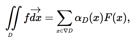
where $\nabla D$ is the set of corners of $D$, and $\alpha_{D}$ accepts values in $\left\{ 0,\pm1\right\} $ and is determined according to the type of corner that $x$ belongs to.

The derivative sign doesn’t reflect trends at cusp points such as corners, therefore it doesn’t classify corner types concisely. In contrast, it turns out that the detachment operator classifies corners (and thus defines the parameter $\alpha_{D}$ coherently) independently of the curve’s parameterization. That’s a multidimensional generalization of our above discussion regarding the relation between both operators. Feel free to interact with the following widget to gain intuition regarding theorem 16. The textboxes toggle the antiderivative at the annotated point, which is reflected in the highlighted domain. Watch the inclusion-exclusion principle in action as the domains finally aggregate to the domain bounded by the vertices. While this theorem is defined over continuous domains, it is limited to generalized rectangular ones. Let’s attempt to alleviate this limitation.


We leverage the detachment to define a novel integration method that extends theorem 16 to non-rectangular domains by combining it with the mean value theorem, as follows. Given a simple closed detachable curve $C$, let $D$ be the region bounded by the curve. Let $R\subseteq D$ be a rectangular domain circumscribed by $C$. Let ${C_i}$ be the sub-curves of $C$ between each pair of its consecutive touching points with $R.$ Let $D_{i}\subset D\backslash R$ be the sub-domain bounded between $C_i$ and $R$. Let $\partial D_i$ be the boundary of $D_i$, and let $\nabla D_{i}$ be the intersection between $D_i$ and the vertices of $R$. According to the mean value theorem in two dimensions, $\forall i:\exists x_{i}\in D_{i}$ such that $\underset{\scriptscriptstyle D_{i}}{\iint}f\overrightarrow{dx}=\beta_{i}f\left(x_{i}\right),$ where $\beta_{i}$ is the area of $D_{i}.$

Our semi-discrete integration method accumulates a linear combination of the function and its antiderivative along the sub-domains $D_{i}$, as follows:

Theorem 17. Let $D\subset\mathbb{R}^{2}$ be a closed, bounded, and connected domain whose edge is detachable. Let $f:\mathbb{R}^{2}\rightarrow\mathbb{R}$ be a function that admits an antiderivative $F.$ Then: $$\underset{\scriptscriptstyle D}{\iint}f\overrightarrow{dx}=\underset{i}{\sum}\left[\overrightarrow{\alpha_{i}}\cdot F\left(\overrightarrow{c_{i}}\right)+\beta_{i}f\left(s_{i}\right)\right],$$where $F\left(\overrightarrow{c_{i}}\right)=\left(F\left(c\right)\,|\,c\in\nabla D_{i}\right)^T$ is the vector of antiderivative values at the vertices of the subdomain $D_{i}$, $\overrightarrow{\alpha_{i}}=\left(\alpha\left(\partial D_{i}^{;},c\right)\,|\,x\in\nabla D_{i}\right)^T$ is a vector containing the results of applying a function $\alpha$ to the detachments of the curve $\partial D_{i}^{;}$ at its vertices $\nabla D_{i}$, and $\beta_i$ is the area of $D_i$, which we incorporate as part of the mean value theorem for integrals along with it matching point in $D_i$ denoted by $s_i$. The function $\alpha$ is constructed within the integration method (see [31]). This formula holds for any detachable division of the curve. We don’t assume the differentiability of the curve’s parameterization, rather only the continuity of the function in $\underset{i}{\bigcup}D_{i}$, for the mean value theorem to hold.
Feel free to gain intuition from the following widget. Initially, the domain is rectangular: $D=R$. Tuning the vertices locations exposes the yellow sub-domains $D_i$, whose areas are $\beta_i$. The integral over $R$ is calculated by aggregating the antiderivative’s value along the vertices of each $D_i$ (the highlighted points in this diagram). The antiderivative values are added to the aggregation with coefficients that are determined by the curve’s detachments at each vertex (the function $\alpha$).


Summary

This was a short Semi-discrete Calculus tour where we just presented the main definitions and results. Hope you’ve learned and enjoyed it. Good luck with your Calculus adventures and stay safe!

References

[1] Dan Alistarh, Demjan Grubic, Jerry Li, Ryota Tomioka, and Milan Vojnovic. Qsgd: Communication-ecient sgd via gradient quantization and encoding. In Advances in Neural Information Processing Systems, pages 1709-1720, 2017.

[2] Marcin Andrychowicz, Misha Denil, Sergio Gomez, Matthew W Hoffman, David Pfau, Tom Schaul, Brendan Shillingford, and Nando De Freitas. Learning to learn by gradient descent by gradient descent. In Advances in neural information processing systems, pages 3981-3989, 2016.

[3] Sven Behnke. Hierarchical neural networks for image interpretation, volume 2766. Springer, 2003.

[4] Jeffrey Byrne. Nested motion descriptors. In Proceedings of the IEEE conference on computer vision and pattern recognition, pages 502-510, 2015.

[5] Zhixiang Chen, Xin Yuan, Jiwen Lu, Qi Tian, and Jie Zhou. Deep hashing via discrepancy minimization. In Proceedings of the IEEE Conference on Computer Vision and Pattern Recognition, pages 6838-6847, 2018.

[6] Kai Fan. Unifying the stochastic spectral descent for restricted boltzmann machines with bernoulli or gaussian inputs. arXiv preprint arXiv:1703.09766, 2017.

[7] Mathias Gallardo, Daniel Pizarro, Adrien Bartoli, and Toby Collins. Shape-from-template in flatland. In Proceedings of the IEEE Conference on Computer Vision and Pattern Recognition, pages 2847-2854, 2015.

[8] Yaroslav Ganin and Victor Lempitsky. Unsupervised domain adaptation by backpropagation. In International conference on machine learning, pages
1180-1189, 2015.

[9] Amirata Ghorbani, Abubakar Abid, and James Zou. Interpretation of neural networks is fragile. In Proceedings of the AAAI Conference on Artificial Intelligence, volume 33, pages 3681-3688, 2019.

[10] Ian J Goodfellow, Jonathon Shlens, and Christian Szegedy. Explaining and harnessing adversarial examples. arXiv preprint arXiv:1412.6572, 2014.

[11] Zhe Hu, Sunghyun Cho, Jue Wang, and Ming-Hsuan Yang. Deblurring low-light images with light streaks. In Proceedings of the IEEE Conference on Computer Vision and Pattern Recognition, pages 3382-3389, 2014.

[12] Itay Hubara, Matthieu Courbariaux, Daniel Soudry, Ran El-Yaniv, and Yoshua Bengio. Quantized neural networks: Training neural networks with low precision weights and activations. The Journal of Machine Learning Research, 18(1):6869-6898, 2017.

[13] Xiangyu Kong, Bo Xin, Yizhou Wang, and Gang Hua. Collaborative deep reinforcement learning for joint object search. In Proceedings of the IEEE Conference on Computer Vision and Pattern Recognition, pages 1695-1704, 2017.

[14] Alexey Kurakin, Ian Goodfellow, and Samy Bengio. Adversarial examples in the physical world. arXiv preprint arXiv:1607.02533, 2016.

[15] Jean Lafond, Hoi-To Wai, and Eric Moulines. On the online frankwolfe algorithms for convex and non-convex optimizations. arXiv preprint arXiv:1510.01171, 2015.

[16] Debang Li, Huikai Wu, Junge Zhang, and Kaiqi Huang. A2-rl: Aesthetics aware reinforcement learning for image cropping. In Proceedings of the IEEE Conference on Computer Vision and Pattern Recognition, pages 8193-8201, 2018.

[17] Wei Li and Xiaogang Wang. Locally aligned feature transforms across views. In Proceedings of the IEEE conference on computer vision and pattern recognition, pages 3594-3601, 2013.

[18] Li Liu, Ling Shao, Fumin Shen, and Mengyang Yu. Discretely coding semantic rank orders for supervised image hashing. In Proceedings of the IEEE conference on computer vision and pattern recognition, pages 1425-1434, 2017.

[19] Seyed-Mohsen Moosavi-Dezfooli, Alhussein Fawzi, and Pascal Frossard. Deepfool: a simple and accurate method to fool deep neural networks. In Proceedings of the IEEE conference on computer vision and pattern recognition, pages 2574-2582, 2016.

[20] Seyed-Mohsen Moosavi-Dezfooli, Alhussein Fawzi, Jonathan Uesato, and Pascal Frossard. Robustness via curvature regularization, and vice versa. In Proceedings of the IEEE Conference on Computer Vision and Pattern Recognition, pages 9078-9086, 2019.

[21] Ali Mousavi, Arian Maleki, Richard G Baraniuk, et al. Consistent parameter estimation for lasso and approximate message passing. The Annals of Statistics, 46(1):119-148, 2018.

[22] Vidhya Navalpakkam and Laurent Itti. Optimal cue selection strategy. In Advances in neural information processing systems, pages 987-994, 2006.

[23] Jinshan Pan, Zhouchen Lin, Zhixun Su, and Ming-Hsuan Yang. Robust kernel estimation with outliers handling for image deblurring. In Proceedings of the IEEE Conference on Computer Vision and Pattern Recognition, pages 2800-2808, 2016.

[24] Nicolas Papernot, Patrick McDaniel, Ananthram Swami, and Richard Harang. Crafting adversarial input sequences for recurrent neural networks. In MILCOM 2016-2016 IEEE Military Communications Conference, pages 49-54. IEEE, 2016.

[25] Ben Poole, Subhaneil Lahiri, Maithra Raghu, Jascha Sohl-Dickstein, and Surya Ganguli. Exponential expressivity in deep neural networks through transient chaos. In Advances in neural information processing systems, pages 3360-3368, 2016.

[26] Aaditya Ramdas and Aarti Singh. Algorithmic connections between active learning and stochastic convex optimization. In International Conference on Algorithmic Learning Theory, pages 339-353. Springer, 2013.

[27] Miriam Redi, Neil O’Hare, Rossano Schifanella, Michele Trevisiol, and Alejandro Jaimes. 6 seconds of sound and vision: Creativity in micro-videos. In Proceedings of the IEEE Conference on Computer Vision and Pattern Recognition, pages 4272-4279, 2014.

[28] Jaakko Riihimäki and Aki Vehtari. Gaussian processes with monotonicity information. In Proceedings of the thirteenth international conference on artificial intelligence and statistics, pages 645-652, 2010.

[29] Swami Sankaranarayanan, Arpit Jain, Rama Chellappa, and Ser Nam Lim. Regularizing deep networks using efficient layerwise adversarial training. In Thirty-Second AAAI Conference on Artificial Intelligence, 2018.

[30] Hee Seok Lee and Kuoung Mu Lee. Simultaneous super-resolution of depth and images using a single camera. In Proceedings of the IEEE Conference on Computer Vision and Pattern Recognition, pages 281-288, 2013.

[31] Amir Shachar. Applying semi-discrete operators to calculus. arXiv preprint arXiv:1012.5751, 2010.

[32] Eero Siivola, Aki Vehtari, Jarno Vanhatalo, Javier González, and Michael Riis Andersen. Correcting boundary over-exploration deficiencies in bayesian optimization with virtual derivative sign observations. In 2018 IEEE 28th International Workshop on Machine Learning for Signal Processing (MLSP), pages 1-6. IEEE, 2018.

[33] Michel Silva, Washington Ramos, Joao Ferreira, Felipe Chamone, Mario Campos, and Erickson R Nascimento. A weighted sparse sampling and smoothing frame transition approach for semantic fast-forward first-person videos. In Proceedings of the IEEE Conference on Computer Vision and Pattern Recognition, pages 2383-2392, 2018.

[34] Yansong Tang, Yi Tian, Jiwen Lu, Peiyang Li, and Jie Zhou. Deep progressive reinforcement learning for skeleton-based action recognition. In Proceedings of the IEEE Conference on Computer Vision and Pattern Recognition, pages 5323-5332, 2018.

[35] Roberto Tron and Kostas Daniilidis. On the quotient representation for the essential manifold. In Proceedings of the IEEE Conference on Computer Vision and Pattern Recognition, pages 1574-1581, 2014.

[36] Paul Viola and Michael Jones. Rapid object detection using a boosted cascade of simple features. In Proceedings of the 2001 IEEE computer society conference on computer vision and pattern recognition. CVPR 2001, volume 1, pages II. IEEE, 2001.

[37] Haohan Wang and Bhiksha Raj. On the origin of deep learning. arXiv preprint arXiv:1702.07800, 2017.

[38] Xiaogang Wang, Gianfranco Doretto, Thomas Sebastian, Jens Rittscher, and Peter Tu. Shape and appearance context modeling. In 2007 ieee 11th international conference on computer vision, pages 18. Ieee, 2007.

[39] Wei Wen, Cong Xu, Feng Yan, Chunpeng Wu, Yandan Wang, Yiran Chen, and Hai Li. Terngrad: Ternary gradients to reduce communication in distributed deep learning. In Advances in neural information processing systems, pages 1509-1519, 2017.

[40] Shaodan Zhai, Tian Xia, Ming Tan, and Shaojun Wang. Direct 0-1 loss minimization and margin maximization with boosting. In Advances in Neural Information Processing Systems, pages 872-880, 2013.

[41] Yu Zhu, Yanning Zhang, Boyan Bonev, and Alan L Yuille. Modeling deformable gradient compositions for single-image super-resolution. In Proceedings of the IEEE Conference on Computer Vision and Pattern Recognition, pages 5417-5425, 2015.

[42] Sachin Ravi and Hugo Larochelle. Optimization as a model for few-shot learning. 2016.

[43] Bernhard Riemann. Uber die Darstellbarkeit einer Function durch eine trigonometrische Reihe, Gott. Abh. (1854/1868); also in: Gesammelte Mathematische Werke, Springer-Verlag, Berlin 1990, 259–296.


Interested in learning more about the NICE Actimize Data Science team?
Get in Touch